7 Data Reshaping, Joining, and Iteration

7.1 Learning Objectives

By the end of this chapter, you will be able to:

Understand and apply tidy data principles to organize datasets effectively
Reshape data between wide and long formats using pivot_longer() and pivot_wider()
Split and combine columns using separate() and unite()
Join multiple datasets using SQL-style joins (left_join(), inner_join(), etc.)
Understand when to use different join types and filtering joins
Bind datasets together with bind_rows() and bind_cols()
Use functional programming with purrr::map() for iteration
Work with list columns and nested data structures

7.2 Introduction

In previous chapters, you learned to manipulate single datasets with dplyr. Real-world analysis often requires: - Reshaping data between different formats - Combining multiple related datasets - Iterating operations across many groups or files

This chapter teaches these essential data wrangling skills using tidyr for reshaping and purrr for iteration.

7.2.1 Setup

library(tidyverse)  # Includes tidyr, dplyr, purrr
library(readxl)     # For reading Excel files

# Set default theme for plots
theme_set(theme_minimal())

7.3 Tidy Data Principles

7.3.1 What is Tidy Data?

Tidy data follows three interrelated rules:

Each variable forms a column
Each observation forms a row
Each type of observational unit forms a table

Hadley Wickham’s Tidy Data

The concept of tidy data comes from Hadley Wickham’s 2014 paper in the Journal of Statistical Software. Tidy data makes analysis easier because: - Variables are easy to access as columns - Observations are easy to filter as rows - Most tidyverse functions expect tidy data

7.3.2 Tidy vs Untidy Data

Example 1: Animal weight measurements

Untidy (wide format):

# Each time point is a separate column
untidy_weights <- tibble(
  animal_id = c("A001", "A002", "A003"),
  week_0 = c(45, 48, 43),
  week_4 = c(52, 54, 50),
  week_8 = c(58, 61, 56),
  week_12 = c(64, 67, 62)
)

untidy_weights

# A tibble: 3 × 5
  animal_id week_0 week_4 week_8 week_12
  <chr>      <dbl>  <dbl>  <dbl>   <dbl>
1 A001          45     52     58      64
2 A002          48     54     61      67
3 A003          43     50     56      62

Tidy (long format):

# Each observation (animal × time) is a separate row
tidy_weights <- tibble(
  animal_id = rep(c("A001", "A002", "A003"), each = 4),
  week = rep(c(0, 4, 8, 12), times = 3),
  weight_kg = c(45, 52, 58, 64,  # A001
                48, 54, 61, 67,  # A002
                43, 50, 56, 62)  # A003
)

tidy_weights

# A tibble: 12 × 3
   animal_id  week weight_kg
   <chr>     <dbl>     <dbl>
 1 A001          0        45
 2 A001          4        52
 3 A001          8        58
 4 A001         12        64
 5 A002          0        48
 6 A002          4        54
 7 A002          8        61
 8 A002         12        67
 9 A003          0        43
10 A003          4        50
11 A003          8        56
12 A003         12        62

Why is tidy better?

# Easy to plot with ggplot2
ggplot(tidy_weights, aes(x = week, y = weight_kg, color = animal_id)) +
  geom_line(linewidth = 1) +
  geom_point(size = 3) +
  labs(title = "Animal Growth Curves",
       x = "Week",
       y = "Weight (kg)",
       color = "Animal ID")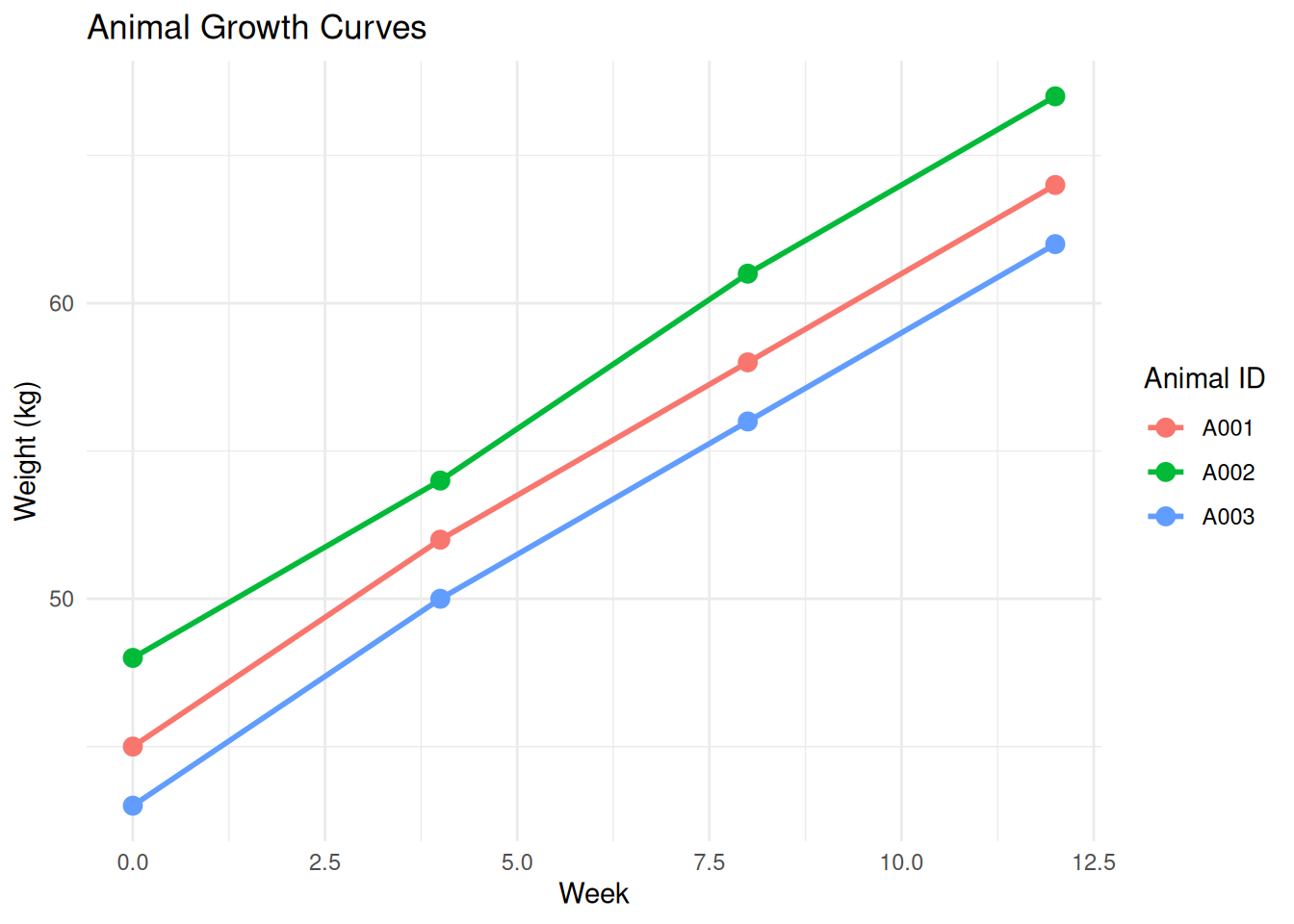

# Easy to calculate summaries
tidy_weights %>%
  group_by(week) %>%
  summarise(
    mean_weight = mean(weight_kg),
    sd_weight = sd(weight_kg)
  )

# A tibble: 4 × 3
   week mean_weight sd_weight
  <dbl>       <dbl>     <dbl>
1     0        45.3      2.52
2     4        52        2   
3     8        58.3      2.52
4    12        64.3      2.52

7.3.3 Common Messy Data Problems

Column headers are values, not variable names (like week_0, week_4)
Multiple variables in one column (like “Holstein-Male”)
Variables stored in both rows and columns
Multiple types of observational units in the same table
Single observational unit stored in multiple tables

This chapter teaches how to fix these problems.

7.4 Data Reshaping with tidyr

7.4.1 `pivot_longer()`: Wide to Long

pivot_longer() transforms wide data (many columns) into long data (many rows).

Basic syntax:

pivot_longer(
  data,
  cols = <columns to pivot>,
  names_to = "<name for new column with old column names>",
  values_to = "<name for new column with values>"
)

7.4.1.1 Example: Pivoting Weight Measurements

# Start with wide format
wide_weights <- tibble(
  animal_id = c("A001", "A002", "A003"),
  breed = c("Holstein", "Jersey", "Angus"),
  week_0 = c(45, 42, 48),
  week_4 = c(52, 48, 54),
  week_8 = c(58, 54, 61)
)

wide_weights

# A tibble: 3 × 5
  animal_id breed    week_0 week_4 week_8
  <chr>     <chr>     <dbl>  <dbl>  <dbl>
1 A001      Holstein     45     52     58
2 A002      Jersey       42     48     54
3 A003      Angus        48     54     61

# Pivot to long format
long_weights <- wide_weights %>%
  pivot_longer(
    cols = starts_with("week"),
    names_to = "time_point",
    values_to = "weight_kg"
  )

long_weights

# A tibble: 9 × 4
  animal_id breed    time_point weight_kg
  <chr>     <chr>    <chr>          <dbl>
1 A001      Holstein week_0            45
2 A001      Holstein week_4            52
3 A001      Holstein week_8            58
4 A002      Jersey   week_0            42
5 A002      Jersey   week_4            48
6 A002      Jersey   week_8            54
7 A003      Angus    week_0            48
8 A003      Angus    week_4            54
9 A003      Angus    week_8            61

7.4.1.2 Selecting Columns to Pivot

Multiple ways to specify which columns to pivot:

# By name
wide_weights %>%
  pivot_longer(
    cols = c(week_0, week_4, week_8),
    names_to = "time_point",
    values_to = "weight_kg"
  )

# A tibble: 9 × 4
  animal_id breed    time_point weight_kg
  <chr>     <chr>    <chr>          <dbl>
1 A001      Holstein week_0            45
2 A001      Holstein week_4            52
3 A001      Holstein week_8            58
4 A002      Jersey   week_0            42
5 A002      Jersey   week_4            48
6 A002      Jersey   week_8            54
7 A003      Angus    week_0            48
8 A003      Angus    week_4            54
9 A003      Angus    week_8            61

# By position
wide_weights %>%
  pivot_longer(
    cols = 3:5,
    names_to = "time_point",
    values_to = "weight_kg"
  )

# A tibble: 9 × 4
  animal_id breed    time_point weight_kg
  <chr>     <chr>    <chr>          <dbl>
1 A001      Holstein week_0            45
2 A001      Holstein week_4            52
3 A001      Holstein week_8            58
4 A002      Jersey   week_0            42
5 A002      Jersey   week_4            48
6 A002      Jersey   week_8            54
7 A003      Angus    week_0            48
8 A003      Angus    week_4            54
9 A003      Angus    week_8            61

# Everything except ID columns
wide_weights %>%
  pivot_longer(
    cols = -c(animal_id, breed),
    names_to = "time_point",
    values_to = "weight_kg"
  )

# A tibble: 9 × 4
  animal_id breed    time_point weight_kg
  <chr>     <chr>    <chr>          <dbl>
1 A001      Holstein week_0            45
2 A001      Holstein week_4            52
3 A001      Holstein week_8            58
4 A002      Jersey   week_0            42
5 A002      Jersey   week_4            48
6 A002      Jersey   week_8            54
7 A003      Angus    week_0            48
8 A003      Angus    week_4            54
9 A003      Angus    week_8            61

7.4.1.3 Cleaning Column Names During Pivot

Use names_prefix to remove prefixes and names_transform to change types:

# Remove "week_" prefix and convert to numeric
wide_weights %>%
  pivot_longer(
    cols = starts_with("week"),
    names_to = "week",
    values_to = "weight_kg",
    names_prefix = "week_",
    names_transform = list(week = as.integer)
  )

# A tibble: 9 × 4
  animal_id breed     week weight_kg
  <chr>     <chr>    <int>     <dbl>
1 A001      Holstein     0        45
2 A001      Holstein     4        52
3 A001      Holstein     8        58
4 A002      Jersey       0        42
5 A002      Jersey       4        48
6 A002      Jersey       8        54
7 A003      Angus        0        48
8 A003      Angus        4        54
9 A003      Angus        8        61

7.4.1.4 Multiple Value Columns

What if you have multiple measurements at each time point?

# Wide data with multiple measurements
wide_multi <- tibble(
  animal_id = c("A001", "A002"),
  weight_week0 = c(45, 42),
  weight_week4 = c(52, 48),
  height_week0 = c(80, 78),
  height_week4 = c(85, 82)
)

wide_multi

# A tibble: 2 × 5
  animal_id weight_week0 weight_week4 height_week0 height_week4
  <chr>            <dbl>        <dbl>        <dbl>        <dbl>
1 A001                45           52           80           85
2 A002                42           48           78           82

# Alternative: create separate columns for each measurement
wide_multi %>%
  pivot_longer(
    cols = -animal_id,
    names_to = c(".value", "week"),
    names_pattern = "(.+)_week(.+)"
  )

# A tibble: 4 × 4
  animal_id week  weight height
  <chr>     <chr>  <dbl>  <dbl>
1 A001      0         45     80
2 A001      4         52     85
3 A002      0         42     78
4 A002      4         48     82

names_pattern with Regular Expressions

Use names_pattern with regex to extract parts of column names: - .+ matches one or more characters - (.+) creates a capture group - week(.+) matches “week” followed by captured characters

7.4.2 `pivot_wider()`: Long to Wide

pivot_wider() transforms long data (many rows) into wide data (many columns). It’s the opposite of pivot_longer().

Basic syntax:

pivot_wider(
  data,
  names_from = <column with names for new columns>,
  values_from = <column with values to fill new columns>
)

7.4.2.1 Example: Creating a Summary Table

# Long format data
animals_long <- tibble(
  animal_id = rep(c("A001", "A002", "A003"), each = 3),
  breed = rep(c("Holstein", "Jersey", "Angus"), each = 3),
  treatment = rep(c("Control", "Treatment_A", "Treatment_B"), times = 3),
  weight_gain_kg = c(15, 22, 18, 12, 18, 15, 16, 21, 17)
)

animals_long

# A tibble: 9 × 4
  animal_id breed    treatment   weight_gain_kg
  <chr>     <chr>    <chr>                <dbl>
1 A001      Holstein Control                 15
2 A001      Holstein Treatment_A             22
3 A001      Holstein Treatment_B             18
4 A002      Jersey   Control                 12
5 A002      Jersey   Treatment_A             18
6 A002      Jersey   Treatment_B             15
7 A003      Angus    Control                 16
8 A003      Angus    Treatment_A             21
9 A003      Angus    Treatment_B             17

# Pivot wider: treatments become columns
animals_wide <- animals_long %>%
  pivot_wider(
    names_from = treatment,
    values_from = weight_gain_kg
  )

animals_wide

# A tibble: 3 × 5
  animal_id breed    Control Treatment_A Treatment_B
  <chr>     <chr>      <dbl>       <dbl>       <dbl>
1 A001      Holstein      15          22          18
2 A002      Jersey        12          18          15
3 A003      Angus         16          21          17

7.4.2.2 Handling Multiple Value Columns

# Long data with multiple measurements
measurements_long <- tibble(
  animal_id = rep(c("A001", "A002"), each = 4),
  week = rep(c(0, 4, 8, 12), times = 2),
  weight_kg = c(45, 52, 58, 64, 42, 48, 54, 60),
  height_cm = c(80, 85, 88, 91, 78, 82, 85, 88)
)

measurements_long

# A tibble: 8 × 4
  animal_id  week weight_kg height_cm
  <chr>     <dbl>     <dbl>     <dbl>
1 A001          0        45        80
2 A001          4        52        85
3 A001          8        58        88
4 A001         12        64        91
5 A002          0        42        78
6 A002          4        48        82
7 A002          8        54        85
8 A002         12        60        88

# Pivot wider: weeks become columns for each measurement
measurements_long %>%
  pivot_wider(
    names_from = week,
    values_from = c(weight_kg, height_cm),
    names_glue = "{.value}_week{week}"
  )

# A tibble: 2 × 9
  animal_id weight_kg_week0 weight_kg_week4 weight_kg_week8 weight_kg_week12
  <chr>               <dbl>           <dbl>           <dbl>            <dbl>
1 A001                   45              52              58               64
2 A002                   42              48              54               60
# ℹ 4 more variables: height_cm_week0 <dbl>, height_cm_week4 <dbl>,
#   height_cm_week8 <dbl>, height_cm_week12 <dbl>

7.4.2.3 Dealing with Duplicates

What if you have duplicate id-time combinations?

# Data with duplicates
duplicated_data <- tibble(
  animal_id = c("A001", "A001", "A002", "A002"),
  week = c(0, 0, 0, 0),  # Same animal measured twice
  weight_kg = c(45, 46, 42, 43)
)

duplicated_data

# A tibble: 4 × 3
  animal_id  week weight_kg
  <chr>     <dbl>     <dbl>
1 A001          0        45
2 A001          0        46
3 A002          0        42
4 A002          0        43

# Summarize first to remove duplicates
duplicated_data %>%
  group_by(animal_id, week) %>%
  summarise(weight_kg = mean(weight_kg), .groups = "drop") %>%
  pivot_wider(
    names_from = week,
    values_from = weight_kg
  )

# A tibble: 2 × 2
  animal_id   `0`
  <chr>     <dbl>
1 A001       45.5
2 A002       42.5

Watch Out for Duplicates!

pivot_wider() creates list-columns when there are multiple values for the same id × names_from combination. Either: - Summarize first (take mean, max, etc.) - Keep as list-column and unnest() later - Check your data for unexpected duplicates

7.4.3 `separate()`: Split One Column into Many

separate() splits a single column into multiple columns based on a separator.

Basic syntax:

separate(
  data,
  col = <column to split>,
  into = c("<new_col1>", "<new_col2>"),
  sep = "<separator>"
)

7.4.3.1 Example: Splitting Composite IDs

# Data with composite identifiers
animals_composite <- tibble(
  animal_id = c("Holstein_M_001", "Jersey_F_002", "Angus_M_003"),
  weight_kg = c(550, 420, 580)
)

animals_composite

# A tibble: 3 × 2
  animal_id      weight_kg
  <chr>              <dbl>
1 Holstein_M_001       550
2 Jersey_F_002         420
3 Angus_M_003          580

# Separate into components
animals_composite %>%
  separate(
    col = animal_id,
    into = c("breed", "sex", "id_number"),
    sep = "_"
  )

# A tibble: 3 × 4
  breed    sex   id_number weight_kg
  <chr>    <chr> <chr>         <dbl>
1 Holstein M     001             550
2 Jersey   F     002             420
3 Angus    M     003             580

7.4.3.2 Automatic Type Conversion

# Separate and convert types automatically
animals_composite %>%
  separate(
    col = animal_id,
    into = c("breed", "sex", "id_number"),
    sep = "_",
    convert = TRUE  # Automatically converts to appropriate types
  )

# A tibble: 3 × 4
  breed    sex   id_number weight_kg
  <chr>    <chr>     <int>     <dbl>
1 Holstein M             1       550
2 Jersey   F             2       420
3 Angus    M             3       580

7.4.3.3 Keeping the Original Column

# Keep original column
animals_composite %>%
  separate(
    col = animal_id,
    into = c("breed", "sex", "id_number"),
    sep = "_",
    remove = FALSE  # Don't remove original column
  )

# A tibble: 3 × 5
  animal_id      breed    sex   id_number weight_kg
  <chr>          <chr>    <chr> <chr>         <dbl>
1 Holstein_M_001 Holstein M     001             550
2 Jersey_F_002   Jersey   F     002             420
3 Angus_M_003    Angus    M     003             580

7.4.4 `unite()`: Combine Columns into One

unite() is the opposite of separate() — it combines multiple columns into one.

Basic syntax:

unite(
  data,
  col = "<new_column_name>",
  ...,
  sep = "<separator>"
)

7.4.4.1 Example: Creating Unique IDs

# Separate columns
animals_separated <- tibble(
  farm = c("North", "South", "East"),
  breed = c("Holstein", "Jersey", "Angus"),
  id_num = c(1, 2, 3),
  weight_kg = c(550, 420, 580)
)

animals_separated

# A tibble: 3 × 4
  farm  breed    id_num weight_kg
  <chr> <chr>     <dbl>     <dbl>
1 North Holstein      1       550
2 South Jersey        2       420
3 East  Angus         3       580

# Unite into single ID
animals_separated %>%
  unite(
    col = "animal_id",
    farm, breed, id_num,
    sep = "_"
  )

# A tibble: 3 × 2
  animal_id        weight_kg
  <chr>                <dbl>
1 North_Holstein_1       550
2 South_Jersey_2         420
3 East_Angus_3           580

7.4.4.2 Keeping Original Columns

# Keep original columns
animals_separated %>%
  unite(
    col = "animal_id",
    farm, breed, id_num,
    sep = "_",
    remove = FALSE
  )

# A tibble: 3 × 5
  animal_id        farm  breed    id_num weight_kg
  <chr>            <chr> <chr>     <dbl>     <dbl>
1 North_Holstein_1 North Holstein      1       550
2 South_Jersey_2   South Jersey        2       420
3 East_Angus_3     East  Angus         3       580

7.4.5 When to Use Each Function

Goal	Function	Example
Many columns → few rows	`pivot_longer()`	week_0, week_4, week_8 → week column
Few columns → many rows	`pivot_wider()`	week column → week_0, week_4, week_8
One column → many columns	`separate()`	“Holstein_M_001” → breed, sex, id
Many columns → one column	`unite()`	breed, sex, id → “Holstein_M_001”

7.5 Joining Datasets

In real-world analysis, data is often spread across multiple tables. Joins combine tables based on shared keys.

7.5.1 Relational Data Example

# Table 1: Animal information
animals <- tibble(
  animal_id = c("A001", "A002", "A003", "A004"),
  breed = c("Holstein", "Jersey", "Angus", "Holstein"),
  birth_date = as.Date(c("2023-01-15", "2023-02-20", "2023-01-10", "2023-03-05"))
)

# Table 2: Weight records
weights <- tibble(
  animal_id = c("A001", "A001", "A002", "A002", "A005"),
  date = as.Date(c("2023-06-01", "2023-09-01", "2023-06-01", "2023-09-01", "2023-06-01")),
  weight_kg = c(180, 220, 150, 185, 200)
)

# Table 3: Treatment assignments
treatments <- tibble(
  animal_id = c("A001", "A002", "A003"),
  treatment = c("Control", "Treatment_A", "Treatment_B")
)

animals

# A tibble: 4 × 3
  animal_id breed    birth_date
  <chr>     <chr>    <date>    
1 A001      Holstein 2023-01-15
2 A002      Jersey   2023-02-20
3 A003      Angus    2023-01-10
4 A004      Holstein 2023-03-05

weights

# A tibble: 5 × 3
  animal_id date       weight_kg
  <chr>     <date>         <dbl>
1 A001      2023-06-01       180
2 A001      2023-09-01       220
3 A002      2023-06-01       150
4 A002      2023-09-01       185
5 A005      2023-06-01       200

treatments

# A tibble: 3 × 2
  animal_id treatment  
  <chr>     <chr>      
1 A001      Control    
2 A002      Treatment_A
3 A003      Treatment_B

7.5.2 Types of Joins

7.5.2.1 Mutating Joins: Add Columns

Visual representation:

flowchart TD
    A[Mutating Joins<br/>Add columns from y to x] --> B[left_join]
    A --> C[right_join]
    A --> D[inner_join]
    A --> E[full_join]

    B --> B1[Keep all x rows<br/>Add matching y columns]
    C --> C1[Keep all y rows<br/>Add matching x columns]
    D --> D1[Keep only matching rows<br/>from both x and y]
    E --> E1[Keep all rows<br/>from both x and y]

7.5.3 `left_join()`: Keep All Left Rows

Venn Diagram concept: All of LEFT + matching from RIGHT

# Left join: keep all animals, add treatment info
animals %>%
  left_join(treatments, by = "animal_id")

# A tibble: 4 × 4
  animal_id breed    birth_date treatment  
  <chr>     <chr>    <date>     <chr>      
1 A001      Holstein 2023-01-15 Control    
2 A002      Jersey   2023-02-20 Treatment_A
3 A003      Angus    2023-01-10 Treatment_B
4 A004      Holstein 2023-03-05 <NA>

Notice: - All 4 animals kept (even A004 with no treatment) - A004 gets NA for treatment - Unmatched rows from treatments (if any) are dropped

7.5.3.1 Use `left_join()` when:

You want to add information to your main table
You want to keep all rows from the main table
Missing matches should be NA

7.5.4 `right_join()`: Keep All Right Rows

Venn Diagram concept: All of RIGHT + matching from LEFT

# Right join: keep all treatments, add animal info
animals %>%
  right_join(treatments, by = "animal_id")

# A tibble: 3 × 4
  animal_id breed    birth_date treatment  
  <chr>     <chr>    <date>     <chr>      
1 A001      Holstein 2023-01-15 Control    
2 A002      Jersey   2023-02-20 Treatment_A
3 A003      Angus    2023-01-10 Treatment_B

right_join() is Rarely Used

right_join(x, y) gives the same result as left_join(y, x). Most people prefer to use left_join() and think about the “main” table being on the left.

# These are equivalent:
animals %>% right_join(treatments)
treatments %>% left_join(animals)

7.5.5 `inner_join()`: Keep Only Matching Rows

Venn Diagram concept: Only the INTERSECTION

# Inner join: keep only animals with treatments
animals %>%
  inner_join(treatments, by = "animal_id")

# A tibble: 3 × 4
  animal_id breed    birth_date treatment  
  <chr>     <chr>    <date>     <chr>      
1 A001      Holstein 2023-01-15 Control    
2 A002      Jersey   2023-02-20 Treatment_A
3 A003      Angus    2023-01-10 Treatment_B

Notice: - Only 3 animals kept (A001, A002, A003) - A004 dropped (no treatment) - Perfect when you only want complete cases

7.5.5.1 Use `inner_join()` when:

You only want rows that match in both tables
Unmatched rows should be excluded
You’re analyzing complete cases only

7.5.6 `full_join()`: Keep All Rows from Both

Venn Diagram concept: UNION of LEFT and RIGHT

# Full join: keep everything
animals %>%
  full_join(treatments, by = "animal_id")

# A tibble: 4 × 4
  animal_id breed    birth_date treatment  
  <chr>     <chr>    <date>     <chr>      
1 A001      Holstein 2023-01-15 Control    
2 A002      Jersey   2023-02-20 Treatment_A
3 A003      Angus    2023-01-10 Treatment_B
4 A004      Holstein 2023-03-05 <NA>

7.5.6.1 Use `full_join()` when:

You want all data from both tables
You want to see what’s missing from each table
You’ll handle NA values later

7.5.7 Joining with Multiple Keys

What if matching requires multiple columns?

# Farm data with state
farms <- tibble(
  farm_name = c("Green Acres", "Sunny Farm", "Green Acres"),
  state = c("Iowa", "Kansas", "Nebraska"),
  size_acres = c(500, 350, 600)
)

# Animal locations
animal_locations <- tibble(
  animal_id = c("A001", "A002", "A003"),
  farm_name = c("Green Acres", "Sunny Farm", "Green Acres"),
  state = c("Iowa", "Kansas", "Iowa")
)

# Join on both farm_name AND state
animal_locations %>%
  left_join(farms, by = c("farm_name", "state"))

# A tibble: 3 × 4
  animal_id farm_name   state  size_acres
  <chr>     <chr>       <chr>       <dbl>
1 A001      Green Acres Iowa          500
2 A002      Sunny Farm  Kansas        350
3 A003      Green Acres Iowa          500

7.5.8 Joining with Different Column Names

# Different ID column names
table1 <- tibble(
  animal_id = c("A001", "A002", "A003"),
  weight_kg = c(180, 150, 200)
)

table2 <- tibble(
  id = c("A001", "A002", "A004"),
  breed = c("Holstein", "Jersey", "Angus")
)

# Specify which columns to join on
table1 %>%
  left_join(table2, by = c("animal_id" = "id"))

# A tibble: 3 × 3
  animal_id weight_kg breed   
  <chr>         <dbl> <chr>   
1 A001            180 Holstein
2 A002            150 Jersey  
3 A003            200 <NA>

7.5.9 Filtering Joins: Filter Rows (Don’t Add Columns)

7.5.9.1 `semi_join()`: Keep Rows with Matches

# Semi join: keep animals that have treatments (but don't add treatment column)
animals %>%
  semi_join(treatments, by = "animal_id")

# A tibble: 3 × 3
  animal_id breed    birth_date
  <chr>     <chr>    <date>    
1 A001      Holstein 2023-01-15
2 A002      Jersey   2023-02-20
3 A003      Angus    2023-01-10

Use semi_join() to answer: “Which x rows have a match in y?”

7.5.9.2 `anti_join()`: Keep Rows WITHOUT Matches

# Anti join: keep animals that DON'T have treatments
animals %>%
  anti_join(treatments, by = "animal_id")

# A tibble: 1 × 3
  animal_id breed    birth_date
  <chr>     <chr>    <date>    
1 A004      Holstein 2023-03-05

Use anti_join() to answer: “Which x rows DON’T have a match in y?”

This is incredibly useful for finding missing data or orphaned records.

7.5.10 Join Summary Table

Join Type	Rows Kept	Columns Added	Use When
`left_join(x, y)`	All from x	From y	Adding info to main table
`right_join(x, y)`	All from y	From x	Rarely used (use left_join instead)
`inner_join(x, y)`	Only matches	From both	Only want complete cases
`full_join(x, y)`	All from both	From both	Keep everything
`semi_join(x, y)`	Matches from x	None	Filter x by presence in y
`anti_join(x, y)`	Non-matches from x	None	Filter x by absence in y

7.5.11 Common Join Problems and Solutions

7.5.11.1 Problem 1: Duplicate Keys

# Multiple weights per animal
weights_dup <- tibble(
  animal_id = c("A001", "A001", "A002"),
  weight_kg = c(180, 185, 150)
)

# Join creates all combinations
animals %>%
  left_join(weights_dup, by = "animal_id")

# A tibble: 5 × 4
  animal_id breed    birth_date weight_kg
  <chr>     <chr>    <date>         <dbl>
1 A001      Holstein 2023-01-15       180
2 A001      Holstein 2023-01-15       185
3 A002      Jersey   2023-02-20       150
4 A003      Angus    2023-01-10        NA
5 A004      Holstein 2023-03-05        NA

Solution: If you only want one weight per animal, summarize first:

weights_dup %>%
  group_by(animal_id) %>%
  summarise(avg_weight_kg = mean(weight_kg), .groups = "drop") %>%
  left_join(animals, ., by = "animal_id")

# A tibble: 4 × 4
  animal_id breed    birth_date avg_weight_kg
  <chr>     <chr>    <date>             <dbl>
1 A001      Holstein 2023-01-15          182.
2 A002      Jersey   2023-02-20          150 
3 A003      Angus    2023-01-10           NA 
4 A004      Holstein 2023-03-05           NA

Always Specify by =

If you don’t specify by, joins use all columns with the same name. This can lead to: - Unintended matches - Silent errors - Confusing results

Best practice: Always explicitly state by = "column_name"

7.5.12 Real-World Example: Combining Multiple Tables

# Start with animals
result <- animals %>%
  # Add treatments
  left_join(treatments, by = "animal_id") %>%
  # Add weights (keeping all weight records)
  left_join(weights, by = "animal_id") %>%
  # Calculate age at weighing
  mutate(
    age_days = as.numeric(date - birth_date),
    .after = date
  )

result

# A tibble: 6 × 7
  animal_id breed    birth_date treatment   date       age_days weight_kg
  <chr>     <chr>    <date>     <chr>       <date>        <dbl>     <dbl>
1 A001      Holstein 2023-01-15 Control     2023-06-01      137       180
2 A001      Holstein 2023-01-15 Control     2023-09-01      229       220
3 A002      Jersey   2023-02-20 Treatment_A 2023-06-01      101       150
4 A002      Jersey   2023-02-20 Treatment_A 2023-09-01      193       185
5 A003      Angus    2023-01-10 Treatment_B NA               NA        NA
6 A004      Holstein 2023-03-05 <NA>        NA               NA        NA

7.6 Binding Datasets

Sometimes you need to combine datasets by stacking (rows) or attaching (columns), not by joining on keys.

7.6.1 `bind_rows()`: Stack Datasets Vertically

Use when you have the same structure in multiple datasets.

# Data from multiple farms
farm_a <- tibble(
  animal_id = c("A001", "A002"),
  weight_kg = c(180, 150),
  farm = "Farm_A"
)

farm_b <- tibble(
  animal_id = c("B001", "B002"),
  weight_kg = c(170, 160),
  farm = "Farm_B"
)

# Stack them
bind_rows(farm_a, farm_b)

# A tibble: 4 × 3
  animal_id weight_kg farm  
  <chr>         <dbl> <chr> 
1 A001            180 Farm_A
2 A002            150 Farm_A
3 B001            170 Farm_B
4 B002            160 Farm_B

7.6.1.1 Handling Missing Columns

# Different columns
df1 <- tibble(animal_id = "A001", weight_kg = 180)
df2 <- tibble(animal_id = "B001", height_cm = 125)

# bind_rows() fills missing columns with NA
bind_rows(df1, df2)

# A tibble: 2 × 3
  animal_id weight_kg height_cm
  <chr>         <dbl>     <dbl>
1 A001            180        NA
2 B001             NA       125

7.6.1.2 Adding Source Identifier

# Or use named list
bind_rows(
  "Iowa" = farm_a,
  "Kansas" = farm_b,
  .id = "state"
)

# A tibble: 4 × 4
  state  animal_id weight_kg farm  
  <chr>  <chr>         <dbl> <chr> 
1 Iowa   A001            180 Farm_A
2 Iowa   A002            150 Farm_A
3 Kansas B001            170 Farm_B
4 Kansas B002            160 Farm_B

7.6.2 `bind_cols()`: Attach Datasets Horizontally

Use bind_cols() with Caution!

bind_cols() simply attaches columns side-by-side based on row position. It does NOT match by keys!

Problems: - No checking if rows actually match - Row order must be identical - Easy to create mismatched data

Better alternative: Use a join with a row number or ID column.

# Two datasets with same row order (risky!)
ids <- tibble(animal_id = c("A001", "A002", "A003"))
weights <- tibble(weight_kg = c(180, 150, 200))

# Attach side-by-side
bind_cols(ids, weights)

# A tibble: 3 × 2
  animal_id weight_kg
  <chr>         <dbl>
1 A001            180
2 A002            150
3 A003            200

# MUCH SAFER: Use mutate instead if they're truly row-aligned
ids %>%
  mutate(weight_kg = weights$weight_kg)

# A tibble: 3 × 2
  animal_id weight_kg
  <chr>         <dbl>
1 A001            180
2 A002            150
3 A003            200

# Or use a proper join if you have keys!

7.6.3 When to Use Binding vs Joining

Use	`bind_rows()`	`bind_cols()`	Join
Same structure, stack vertically	✅	❌	❌
Different farms/time periods	✅	❌	❌
Add columns based on keys	❌	❌	✅
Row-aligned data (same order)	❌	⚠️ Use with caution	❌
Relational data (shared IDs)	❌	❌	✅

7.7 Iteration with purrr

The purrr package provides tools for functional programming — applying functions across elements of a list or vector.

7.7.1 Why Use `map()` Instead of Loops?

# Example: Calculate mean of each column

# Base R loop approach
col_means_loop <- numeric(ncol(mtcars))
for (i in seq_along(mtcars)) {
  col_means_loop[i] <- mean(mtcars[[i]])
}
col_means_loop

 [1]  20.090625   6.187500 230.721875 146.687500   3.596563   3.217250
 [7]  17.848750   0.437500   0.406250   3.687500   2.812500

# purrr approach
col_means_map <- map_dbl(mtcars, mean)
col_means_map

       mpg        cyl       disp         hp       drat         wt       qsec 
 20.090625   6.187500 230.721875 146.687500   3.596563   3.217250  17.848750 
        vs         am       gear       carb 
  0.437500   0.406250   3.687500   2.812500

# They're the same!
all.equal(col_means_loop, col_means_map)

[1] "names for current but not for target"

Benefits of map(): - More concise - Less error-prone (no index management) - Easier to read intent - Consistent return types

When to Use Loops vs map()

Use loops when: - You need to modify objects in place - The operation depends on previous iterations - The logic is complex and loops are clearer

Use map() when: - Applying the same operation to each element - You want consistent output types - You’re working with lists or data frames

7.7.2 Basic `map()` Functions

# Create example data
numbers <- list(
  a = c(1, 2, 3, 4, 5),
  b = c(10, 20, 30),
  c = c(100, 200, 300, 400)
)

# map() returns a list
map(numbers, mean)

$a
[1] 3

$b
[1] 20

$c
[1] 250

# map_dbl() returns a numeric vector
map_dbl(numbers, mean)

  a   b   c 
  3  20 250

# map_chr() returns a character vector
map_chr(numbers, \(x) paste("Mean:", round(mean(x), 1)))

          a           b           c 
  "Mean: 3"  "Mean: 20" "Mean: 250"

# map_int() returns an integer vector
map_int(numbers, length)

a b c 
5 3 4

# map_lgl() returns a logical vector
map_lgl(numbers, \(x) mean(x) > 50)

    a     b     c 
FALSE FALSE  TRUE

7.7.3 `map()` with Data Frames

# Create example animal data
animals_list <- list(
  farm_a = tibble(animal_id = c("A001", "A002"), weight_kg = c(180, 150)),
  farm_b = tibble(animal_id = c("B001", "B002"), weight_kg = c(170, 160)),
  farm_c = tibble(animal_id = c("C001", "C002"), weight_kg = c(190, 165))
)

# Calculate mean weight for each farm
map_dbl(animals_list, \(df) mean(df$weight_kg))

farm_a farm_b farm_c 
 165.0  165.0  177.5

# Count rows in each data frame
map_int(animals_list, nrow)

farm_a farm_b farm_c 
     2      2      2

# Add a new column to each data frame
map(animals_list, \(df) mutate(df, weight_lb = weight_kg * 2.20462))

$farm_a
# A tibble: 2 × 3
  animal_id weight_kg weight_lb
  <chr>         <dbl>     <dbl>
1 A001            180      397.
2 A002            150      331.

$farm_b
# A tibble: 2 × 3
  animal_id weight_kg weight_lb
  <chr>         <dbl>     <dbl>
1 B001            170      375.
2 B002            160      353.

$farm_c
# A tibble: 2 × 3
  animal_id weight_kg weight_lb
  <chr>         <dbl>     <dbl>
1 C001            190      419.
2 C002            165      364.

7.7.4 Anonymous Functions in `map()`

Three ways to write anonymous functions:

numbers <- list(a = 1:5, b = 10:15, c = 20:25)

# 1. Traditional function() syntax
map_dbl(numbers, function(x) mean(x) * 2)

 a  b  c 
 6 25 45

# 2. Formula shorthand with ~ and .x
map_dbl(numbers, ~ mean(.x) * 2)

 a  b  c 
 6 25 45

# 3. Lambda function with \() (R >= 4.1)
map_dbl(numbers, \(x) mean(x) * 2)

 a  b  c 
 6 25 45

All three are equivalent. Use whichever you find most readable.

7.7.5 `map2()`: Iterate Over Two Inputs

When you need to iterate over two vectors/lists in parallel:

# Two vectors to iterate over
weights_kg <- c(180, 150, 200)
prices_per_kg <- c(5, 5.50, 4.80)

# Calculate total value for each animal
map2_dbl(weights_kg, prices_per_kg, \(w, p) w * p)

[1] 900 825 960

# With names
animals <- c("A001", "A002", "A003")
map2_chr(animals, weights_kg, \(id, wt) paste(id, "weighs", wt, "kg"))

[1] "A001 weighs 180 kg" "A002 weighs 150 kg" "A003 weighs 200 kg"

7.7.6 `pmap()`: Iterate Over Many Inputs

For more than two inputs, use pmap():

# Data frame with multiple columns
sales <- tibble(
  animal_id = c("A001", "A002", "A003"),
  weight_kg = c(180, 150, 200),
  price_per_kg = c(5, 5.50, 4.80),
  bonus = c(50, 30, 60)
)

# Calculate total value: (weight * price) + bonus
sales %>%
  mutate(
    total_value = pmap_dbl(
      list(weight_kg, price_per_kg, bonus),
      \(w, p, b) (w * p) + b
    )
  )

# A tibble: 3 × 5
  animal_id weight_kg price_per_kg bonus total_value
  <chr>         <dbl>        <dbl> <dbl>       <dbl>
1 A001            180          5      50         950
2 A002            150          5.5    30         855
3 A003            200          4.8    60        1020

7.7.7 Practical Example: Reading Multiple Files

# Get list of CSV files
file_list <- list.files(path = "data/", pattern = "*.csv", full.names = TRUE)

# Read all files into a list
all_data <- map(file_list, read_csv)

# Combine into single data frame with source file
combined_data <- map(file_list, read_csv) %>%
  set_names(basename(file_list)) %>%
  bind_rows(.id = "source_file")

7.7.8 Handling Errors with `safely()` and `possibly()`

Sometimes operations fail for some elements. Handle errors gracefully:

# Some operations might fail
mixed_list <- list(
  a = c(1, 2, 3),
  b = c("a", "b", "c"),  # This will cause an error with mean()
  c = c(10, 20, 30)
)

# This would error:
# map_dbl(mixed_list, mean)

# Use safely() to catch errors
safe_mean <- safely(mean)
map(mixed_list, safe_mean)

$a
$a$result
[1] 2

$a$error
NULL


$b
$b$result
[1] NA

$b$error
NULL


$c
$c$result
[1] 20

$c$error
NULL

# Use possibly() to return a default value on error
possibly_mean <- possibly(mean, otherwise = NA_real_)
map_dbl(mixed_list, possibly_mean)

 a  b  c 
 2 NA 20

7.8 List Columns and Nested Data

List columns allow you to store complex objects (like data frames) inside data frame cells.

7.8.1 Creating Nested Data

# Example: Group and nest
animals_nested <- tibble(
  animal_id = c("A001", "A002", "A003", "A001", "A002", "A003"),
  week = c(0, 0, 0, 4, 4, 4),
  weight_kg = c(45, 42, 48, 52, 48, 54)
) %>%
  group_by(animal_id) %>%
  nest()

animals_nested

# A tibble: 3 × 2
# Groups:   animal_id [3]
  animal_id data            
  <chr>     <list>          
1 A001      <tibble [2 × 2]>
2 A002      <tibble [2 × 2]>
3 A003      <tibble [2 × 2]>

# Each row now contains a data frame in the 'data' column
animals_nested$data[[1]]  # Data for first animal

# A tibble: 2 × 2
   week weight_kg
  <dbl>     <dbl>
1     0        45
2     4        52

7.8.2 Working with Nested Data

# Calculate statistics for each animal's data
animals_nested %>%
  mutate(
    n_measurements = map_int(data, nrow),
    mean_weight = map_dbl(data, ~mean(.x$weight_kg)),
    weight_gain = map_dbl(data, ~diff(range(.x$weight_kg)))
  )

# A tibble: 3 × 5
# Groups:   animal_id [3]
  animal_id data             n_measurements mean_weight weight_gain
  <chr>     <list>                    <int>       <dbl>       <dbl>
1 A001      <tibble [2 × 2]>              2        48.5           7
2 A002      <tibble [2 × 2]>              2        45             6
3 A003      <tibble [2 × 2]>              2        51             6

7.8.3 Fitting Models to Nested Data

# Create more complete data
set.seed(123)
growth_data <- tibble(
  animal_id = rep(c("A001", "A002", "A003"), each = 5),
  week = rep(c(0, 2, 4, 6, 8), times = 3),
  weight_kg = c(
    45 + (0:4) * 2 + rnorm(5, 0, 1),  # A001
    42 + (0:4) * 1.8 + rnorm(5, 0, 1),  # A002
    48 + (0:4) * 2.2 + rnorm(5, 0, 1)   # A003
  )
)

# Nest by animal
growth_nested <- growth_data %>%
  group_by(animal_id) %>%
  nest()

# Fit linear model to each animal's growth
growth_nested <- growth_nested %>%
  mutate(
    model = map(data, ~lm(weight_kg ~ week, data = .x)),
    growth_rate = map_dbl(model, ~coef(.x)[2])
  )

growth_nested

# A tibble: 3 × 4
# Groups:   animal_id [3]
  animal_id data             model  growth_rate
  <chr>     <list>           <list>       <dbl>
1 A001      <tibble [5 × 2]> <lm>         1.08 
2 A002      <tibble [5 × 2]> <lm>         0.627
3 A003      <tibble [5 × 2]> <lm>         0.910

# Extract coefficients
growth_nested %>%
  select(animal_id, growth_rate)

# A tibble: 3 × 2
# Groups:   animal_id [3]
  animal_id growth_rate
  <chr>           <dbl>
1 A001            1.08 
2 A002            0.627
3 A003            0.910

7.8.4 Unnesting

Convert list columns back to regular rows:

# Unnest data column
growth_nested %>%
  select(animal_id, data) %>%
  unnest(cols = data)

# A tibble: 15 × 3
# Groups:   animal_id [3]
   animal_id  week weight_kg
   <chr>     <dbl>     <dbl>
 1 A001          0      44.4
 2 A001          2      46.8
 3 A001          4      50.6
 4 A001          6      51.1
 5 A001          8      53.1
 6 A002          0      43.7
 7 A002          2      44.3
 8 A002          4      44.3
 9 A002          6      46.7
10 A002          8      48.8
11 A003          0      49.2
12 A003          2      50.6
13 A003          4      52.8
14 A003          6      54.7
15 A003          8      56.2

7.9 Summary

This chapter covered three major topics for advanced data wrangling:

7.9.1 Data Reshaping (tidyr)

pivot_longer(): Wide → Long format
- Convert column names to values
- Stack measurements
pivot_wider(): Long → Wide format
- Create summary tables
- Spread values across columns
separate() & unite(): Split or combine columns
- Extract information from composite columns
- Create unique identifiers

7.9.2 Joining Datasets

Mutating joins (add columns):
- left_join(): Keep all left, add matching right
- inner_join(): Keep only matches
- full_join(): Keep everything
Filtering joins (filter rows):
- semi_join(): Keep rows with matches
- anti_join(): Keep rows without matches
Binding:
- bind_rows(): Stack vertically
- bind_cols(): Attach horizontally (use cautiously)

7.9.3 Iteration (purrr)

map() functions: Apply functions to each element
- map(): Returns list
- map_dbl(), map_chr(), map_int(), map_lgl(): Return vectors
Multiple inputs:
- map2(): Two inputs
- pmap(): Many inputs
List columns: Store complex objects in data frames
- nest(): Create nested data
- unnest(): Expand nested data

7.10 Week 7 Homework: Multi-Table Data Integration

7.10.1 Assignment Overview

You will work with three related datasets about a pig feeding trial. Your task is to reshape, join, and analyze the data using techniques from this chapter.

7.10.2 Part 1: Data Generation (0 points, but required)

Run this code to create your datasets:

library(tidyverse)
set.seed(2024)

# Dataset 1: Pig information
pigs <- tibble(
  pig_id = paste0("P", 1001:1050),
  breed = sample(c("Yorkshire", "Duroc", "Hampshire"), 50, replace = TRUE),
  birth_date = as.Date("2023-03-01") + sample(0:30, 50, replace = TRUE),
  initial_weight_kg = rnorm(50, mean = 8, sd = 1)
)

# Dataset 2: Feed records (wide format - needs reshaping!)
feed_wide <- tibble(
  pig_id = paste0("P", 1001:1050),
  week_1_kg = rnorm(50, mean = 5, sd = 0.5),
  week_2_kg = rnorm(50, mean = 6, sd = 0.6),
  week_3_kg = rnorm(50, mean = 7, sd = 0.7),
  week_4_kg = rnorm(50, mean = 8, sd = 0.8)
)

# Dataset 3: Treatment assignments (some pigs, not all)
treatments <- tibble(
  pig_id = sample(paste0("P", 1001:1050), 40),
  treatment = sample(c("Standard", "HighProtein", "Supplement"), 40, replace = TRUE),
  treatment_start = as.Date("2023-03-15")
)

# Dataset 4: Health records (long format, multiple records per pig)
health <- tibble(
  pig_id = rep(sample(paste0("P", 1001:1050), 30), each = 3),
  check_date = rep(as.Date("2023-03-15") + c(7, 14, 21), times = 30),
  health_score = sample(1:10, 90, replace = TRUE),
  temperature_C = rnorm(90, mean = 39, sd = 0.5)
)

# Save datasets
write_csv(pigs, "pigs.csv")
write_csv(feed_wide, "feed_wide.csv")
write_csv(treatments, "treatments.csv")
write_csv(health, "health.csv")

7.10.3 Part 2: Data Reshaping (25 points)

Task 1 (10 points): Reshape feed_wide from wide to long format - Create columns: pig_id, week, feed_consumed_kg - Convert week to numeric (remove “week_” prefix and “_kg” suffix) - Show first 10 rows

Task 2 (10 points): Create a summary table showing average feed by week - Calculate mean feed consumed for each week - Reshape to wide format where weeks are columns - Add a “total” column with sum across weeks

Task 3 (5 points): In the health dataset, separate check_date into year, month, day

7.10.4 Part 3: Joining Datasets (30 points)

Task 1 (10 points): Create a master dataset - Start with pigs - Add treatment information (keep all pigs) - Add the reshaped feed data (long format) - Show structure and first 15 rows

Task 2 (10 points): Analyze which pigs DON’T have health records - Use an appropriate filtering join - Show pig_id, breed, and initial_weight_kg - How many pigs lack health records?

Task 3 (10 points): Create a complete cases dataset - Only include pigs that have: - Treatment assignments - Feed records for all 4 weeks - At least one health record - How many pigs remain? - What’s the average initial weight?

7.10.5 Part 4: Complex Joins (20 points)

Task 1 (10 points): Calculate total feed consumption per pig - Sum feed_consumed_kg across all weeks for each pig - Join with pig information and treatment - Create a table showing mean total feed by breed and treatment - Which breed × treatment combination consumed most feed?

Task 2 (10 points): Identify treatment effects - Calculate average health_score for each pig - Join with treatment information - Compare average health scores across treatments - Create a visualization (boxplot or violin plot)

7.10.6 Part 5: Iteration with purrr (20 points)

Task 1 (10 points): Calculate summary statistics for each breed - Nest data by breed - Use map() to calculate for each breed: - Number of pigs - Mean initial weight - Mean total feed consumed (if you calculated it in Part 4) - Mean health score (if available) - Unnest results into a summary table

Task 2 (10 points): Fit models to nested data - Nest feed data by pig_id - Fit a linear model of feed_consumed_kg ~ week for each pig - Extract the slope (growth rate of feed consumption) - Which pig has the highest feed growth rate? - Which breed has the highest average feed growth rate?

7.10.7 Part 6: Reflection (5 points)

Write 200-300 words addressing: - Which type of join did you use most and why? - What was the most challenging aspect of reshaping the data? - When did you choose map() vs a loop (if at all)? - What insights did you discover about the pig feeding trial?

7.10.8 Recommended YAML

---
title: "Week 7 Homework: Multi-Table Data Integration"
author: "Your Name"
date: today
format:
  html:
    toc: true
    toc-depth: 3
    code-fold: false
    theme: cosmo
    embed-resources: true
execute:
  warning: false
  message: false
---

7.10.9 Grading Rubric

Part 2: Data Reshaping (25%)
- Correct pivoting to long format (10%)
- Summary table correctly reshaped (10%)
- Date separation correct (5%)
Part 3: Joining Datasets (30%)
- Master dataset correctly created (10%)
- Anti-join to find missing health records (10%)
- Complete cases filtering correct (10%)
Part 4: Complex Joins (20%)
- Total feed calculation and table (10%)
- Treatment effects analysis (10%)
Part 5: Iteration with purrr (20%)
- Nested summaries by breed (10%)
- Model fitting with map (10%)
Part 6: Reflection (5%)
- Thoughtful analysis of methods and insights

7.10.10 Bonus (+10 points)

Create a function that takes a pig_id and returns a plot of their feed consumption over time
Use map() to generate plots for all pigs in one breed
Combine plots using patchwork (from Chapter 6)

7.11 Additional Resources

7.11.1 Required Reading

R for Data Science (2e) - Chapters 19-21 (Joins, Tidy Data, Iteration)
tidyr documentation
purrr documentation
Wickham, H. (2014). “Tidy Data.” Journal of Statistical Software, 59(10). Link

7.1 Learning Objectives

7.2 Introduction

7.2.1 Setup

7.3 Tidy Data Principles

7.3.1 What is Tidy Data?

7.3.2 Tidy vs Untidy Data

7.3.3 Common Messy Data Problems

7.4 Data Reshaping with tidyr

7.4.1 pivot_longer(): Wide to Long

7.4.1.1 Example: Pivoting Weight Measurements

7.4.1.2 Selecting Columns to Pivot

7.4.1.3 Cleaning Column Names During Pivot

7.4.1.4 Multiple Value Columns

7.4.2 pivot_wider(): Long to Wide

7.4.2.1 Example: Creating a Summary Table

7.4.2.2 Handling Multiple Value Columns

7.4.2.3 Dealing with Duplicates

7.4.3 separate(): Split One Column into Many

7.4.3.1 Example: Splitting Composite IDs

7.4.3.2 Automatic Type Conversion

7.4.3.3 Keeping the Original Column

7.4.4 unite(): Combine Columns into One

7.4.4.1 Example: Creating Unique IDs

7.4.4.2 Keeping Original Columns

7.4.5 When to Use Each Function

7.5 Joining Datasets

7.5.1 Relational Data Example

7.5.2 Types of Joins

7.5.2.1 Mutating Joins: Add Columns

7.5.3 left_join(): Keep All Left Rows

7.5.3.1 Use left_join() when:

7.5.4 right_join(): Keep All Right Rows

7.5.5 inner_join(): Keep Only Matching Rows

7.5.5.1 Use inner_join() when:

7.5.6 full_join(): Keep All Rows from Both

7.5.6.1 Use full_join() when:

7.5.7 Joining with Multiple Keys

7.5.8 Joining with Different Column Names

7.5.9 Filtering Joins: Filter Rows (Don’t Add Columns)

7.5.9.1 semi_join(): Keep Rows with Matches

7.5.9.2 anti_join(): Keep Rows WITHOUT Matches

7.5.10 Join Summary Table

7.5.11 Common Join Problems and Solutions

7.5.11.1 Problem 1: Duplicate Keys

7.5.12 Real-World Example: Combining Multiple Tables

7.6 Binding Datasets

7.6.1 bind_rows(): Stack Datasets Vertically

7.6.1.1 Handling Missing Columns

7.6.1.2 Adding Source Identifier

7.6.2 bind_cols(): Attach Datasets Horizontally

7.6.3 When to Use Binding vs Joining

7.7 Iteration with purrr

7.7.1 Why Use map() Instead of Loops?

7.7.2 Basic map() Functions

7.7.3 map() with Data Frames

7.7.4 Anonymous Functions in map()

7.7.5 map2(): Iterate Over Two Inputs

7.7.6 pmap(): Iterate Over Many Inputs

7.7.7 Practical Example: Reading Multiple Files

7.7.8 Handling Errors with safely() and possibly()

7.8 List Columns and Nested Data

7.8.1 Creating Nested Data

7.8.2 Working with Nested Data

7.8.3 Fitting Models to Nested Data

7.8.4 Unnesting

7.9 Summary

7.9.1 Data Reshaping (tidyr)

7.9.2 Joining Datasets

7.9.3 Iteration (purrr)

7.10 Week 7 Homework: Multi-Table Data Integration

7.10.1 Assignment Overview

7.10.2 Part 1: Data Generation (0 points, but required)

7.10.3 Part 2: Data Reshaping (25 points)

7.10.4 Part 3: Joining Datasets (30 points)

7.10.5 Part 4: Complex Joins (20 points)

7.10.6 Part 5: Iteration with purrr (20 points)

7.10.7 Part 6: Reflection (5 points)

7.10.8 Recommended YAML

7.10.9 Grading Rubric

7.10.10 Bonus (+10 points)

7.4.1 `pivot_longer()`: Wide to Long

7.4.2 `pivot_wider()`: Long to Wide

7.4.3 `separate()`: Split One Column into Many

7.4.4 `unite()`: Combine Columns into One

7.5.3 `left_join()`: Keep All Left Rows

7.5.3.1 Use `left_join()` when:

7.5.4 `right_join()`: Keep All Right Rows

7.5.5 `inner_join()`: Keep Only Matching Rows

7.5.5.1 Use `inner_join()` when:

7.5.6 `full_join()`: Keep All Rows from Both

7.5.6.1 Use `full_join()` when:

7.5.9.1 `semi_join()`: Keep Rows with Matches

7.5.9.2 `anti_join()`: Keep Rows WITHOUT Matches

7.6.1 `bind_rows()`: Stack Datasets Vertically

7.6.2 `bind_cols()`: Attach Datasets Horizontally

7.7.1 Why Use `map()` Instead of Loops?

7.7.2 Basic `map()` Functions

7.7.3 `map()` with Data Frames

7.7.4 Anonymous Functions in `map()`

7.7.5 `map2()`: Iterate Over Two Inputs

7.7.6 `pmap()`: Iterate Over Many Inputs

7.7.8 Handling Errors with `safely()` and `possibly()`