Recombination and genetic maps • tidybreed

Every offspring add_offspring() creates receives one gamete from each parent, and each gamete is a recombined copy of that parent’s two haplotypes. Linkage disequilibrium, the decay of QTL-marker associations, and the response to genomic selection all follow from how those crossovers are drawn. This article explains the model, shows where the genetic map comes from, and then checks the simulated recombination against the map, so you can see for yourself that the rates are right.

library(tidybreed)
library(dplyr)

The model

For each gamete and each chromosome, add_offspring():

reads the genetic positions (pos_cM) of the chromosome’s loci from the map of the parent making the gamete;
draws the number of crossovers from a Poisson distribution with mean L / 100, where L is the chromosome’s genetic length in cM (the last locus’s pos_cM), i.e. its length in Morgans;
picks the homolog the gamete starts on, 50/50;
places the crossovers uniformly on [0, L]; each locus takes the homolog reached after the crossovers to its left, switching at every one.

Crossovers that fall independently and uniformly are the Haldane model: there is no crossover interference, and two loci d cM apart recombine with probability

$r = \tfrac{1}{2}\left(1 - e^{-2d/100}\right).$

At short distances r is about d / 100; at long distances it approaches 1/2, as for loci on different chromosomes. The same algorithm exists in C++ (used by default) and in R (options(tidybreed.kernel = "r")), and they give bit-identical output for a given seed.

Every gamete draws from its own random stream, keyed on the base seed, the offspring and the parent, so a seeded call gives the same offspring whatever batch_size is.

Where the map comes from

define_genome() places loci evenly along each chromosome (pos_bp) and gives each a genetic position pos_cM = pos_bp / 1e6 * cM_per_Mb. The rate can be one number for the whole genome or one per chromosome:

set.seed(2026)
pop <- open_pop(pop_name = "recombination", db_name = ":memory:") |>
  define_genome(n_loci = 60, n_chr = 3,
                chr_len_Mb = c(150, 100, 80),
                cM_per_Mb  = c(1, 0.5, 1))
#> duckdb keeps downloaded extensions and secrets in a temporary directory:
#> ℹ /tmp/RtmpvmPipF/duckdb
#> This is removed when the R session ends.
#> • Extensions are re-downloaded each session.
#> • Secrets are lost.
#> ℹ Run duckdb(shared_home = TRUE) (or create ~/.duckdb) to keep them (suitable for most users).
#> ℹ Run duckdb(shared_home = FALSE) to accept the temporary directory (and silence this message).
#> ℹ See ?duckdb_storage for details and alternatives.
#> Opened in-memory population 'recombination'
#> 
#> Defined genome: 60 loci across 3 chromosomes | chr lengths (Mb): 1:150, 2:100, 3:80
#>   Tables written: genome_meta, genome_map, ind_haplotype, ind_genotype, ind_crossover, chr_inheritance, chr_recombination, genome_effects, genome_effect_members, genome_effect_member_origins
#>   Views created: genome_effect_terms, genome_effect_loci

# genome_map holds the genetic positions, genome_meta the chromosome of each locus
map <- get_table(pop, "genome_map") |>
  select(locus_id, pos_cM) |>
  collect() |>
  inner_join(get_table(pop, "genome_meta") |> select(locus_id, chr_name) |> collect(),
             by = "locus_id")

map |>
  group_by(chr_name) |>
  summarise(n_loci = n(), first_cM = min(pos_cM), last_cM = max(pos_cM))
#> # A tibble: 3 × 4
#>   chr_name n_loci first_cM last_cM
#>   <chr>     <int>    <dbl>   <dbl>
#> 1 1            20     7.14   143. 
#> 2 2            20     2.38    47.6
#> 3 3            20     3.81    76.2

Chromosome 2 is 100 Mb but only 0.5 cM/Mb, so it is about 50 cM long and averages half a crossover per meiosis. Loci are never placed at the chromosome ends, so the length that matters, the last locus’s position, is a little shorter than chr_len_Mb * cM_per_Mb. A crossover beyond the last locus could not change any allele, so this costs nothing.

genome_map also has sex and line_name columns. A gamete uses, per locus, the most specific row that matches its producing parent: (sex and line), then sex, then line, then the default map. This is how a sex-specific map (female maps are usually longer) or a line-specific map is applied. define_genome() writes only the default map, and there is not yet an exported function to write the others.

Making recombination visible

Recombination is only visible where a parent’s two homologs differ. A cross between two lines makes every locus informative: line A sires mated to line B dams give F1 animals with one A copy and one B copy everywhere, and every allele in ind_haplotype carries its line_origin. In an F1 gamete, each switch from A to B (or back) is a recombination, whatever the alleles are.

Two chromosome rules make the example richer. Chromosome 3 is an X: males inherit only the dam’s copy. Chromosome 2 does not recombine in males (achiasmy, as in Drosophila males).

pop <- pop |>
  define_chromosome("3", offspring_sex = "M", from_parent_1 = 0, from_parent_2 = 1) |>
  define_chromosome("2", parent_sex = "M", recombines = FALSE) |>
  define_founder_haplotypes(n_haplotypes = 10, line_name = "A") |>
  define_founder_haplotypes(n_haplotypes = 10, line_name = "B")
#> Defined chr_inheritance rule for '3' (offspring_sex=M, line_name=NULL): from_parent_1=0, from_parent_2=1
#> Defined chr_recombination rule for '2' (parent_sex=M, line_name=NULL): recombines=FALSE
#> Generating 10 founder haplotypes (method = "uniform")...
#>   Created founder_haplotypes for line 'A' (10 haplotypes x 60 loci)
#> Generating 10 founder haplotypes (method = "uniform")...
#>   Created founder_haplotypes for line 'B' (10 haplotypes x 60 loci)

pop <- pop |>
  get_table("founder_haplotypes") |>
  filter(line_name == "A") |>
  add_founders(n_males = 5, n_females = 0, line_name = "A")
#> Added 5 founders (5 males, 0 females) to line 'A'
pop <- pop |>
  get_table("founder_haplotypes") |>
  filter(line_name == "B") |>
  add_founders(n_males = 0, n_females = 5, line_name = "B")
#> Added 5 founders (0 males, 5 females) to line 'B'

# F1: A sires x B dams
f1 <- tibble(id_parent_1 = paste0("A_", rep(1:5, 4)),
             id_parent_2 = paste0("B_", rep(1:5, 4)),
             sex = rep(c("M", "F"), 10), line_name = "F1")
pop <- add_offspring(pop, f1, seed = 1)
#> Added 20 offspring (base_seed = 1)

# F2: F1 males x F1 females, recording every crossover
n_f2 <- 1500
f1_ids <- get_table(pop, "ind_meta") |> filter(line_name == "F1") |> collect()
f2 <- tibble(
  id_parent_1 = rep(f1_ids$id_ind[f1_ids$sex == "M"], length.out = n_f2),
  id_parent_2 = rep(f1_ids$id_ind[f1_ids$sex == "F"], length.out = n_f2),
  sex = rep(c("M", "F"), length.out = n_f2), line_name = "F2")
pop <- add_offspring(pop, f2, seed = 2, store_crossovers = TRUE)
#> Added 1500 offspring (base_seed = 2)

Here is one F2 animal’s maternal gamete on chromosome 1: the line each allele came from, with the crossovers recorded in ind_crossover as dashed lines.

f2_haps <- get_table(pop, "ind_haplotype") |>
  filter(substr(id_ind, 1, 3) == "F2_") |>
  select(id_ind, parent_origin, locus_id, line_origin) |>
  collect() |>
  inner_join(map, by = "locus_id")

one <- f2_haps |>
  filter(id_ind == "F2_3", parent_origin == 2, chr_name == "1")
xo <- get_table(pop, "ind_crossover") |>
  filter(id_ind == "F2_3", parent_origin == 2, chr_name == "1") |>
  collect()

plot(one$pos_cM, ifelse(one$line_origin == "A", 1, 0), type = "s",
     yaxt = "n", ylim = c(-0.2, 1.2), xlab = "Position (cM)", ylab = "",
     main = "F2_3, maternal gamete, chromosome 1")
points(one$pos_cM, ifelse(one$line_origin == "A", 1, 0), pch = 16, cex = 0.7)
axis(2, at = c(0, 1), labels = c("line B", "line A"), las = 1)
abline(v = xo$pos_cM, lty = 2, col = "grey40")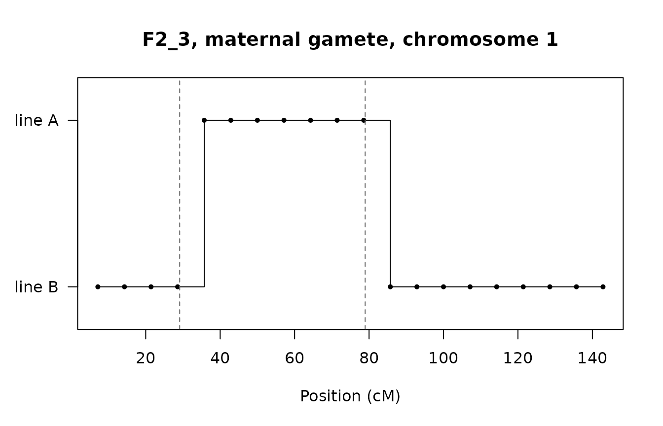

The points are the loci. The line changes at the first locus past each crossover, because only loci are observed: a step falls between two loci exactly when an odd number of crossovers lies between them. Two crossovers between the same pair of loci leave no trace, which is why the recombination fraction is below d / 100 at longer distances.

Checking the rates against the map

For every pair of loci on a chromosome, the observed recombination fraction is the share of gametes whose line changes between the two loci. Plotted against the map distance it should follow the Haldane curve.

# Recombination fraction for every pair of loci on one chromosome, from the
# gametes of one parent sex (parent_origin 1 = sire, 2 = dam)
pair_rates <- function(haps, chr, origin) {
  h <- haps |>
    filter(chr_name == chr, parent_origin == origin) |>
    arrange(id_ind, locus_id)
  pos <- sort(unique(h$pos_cM))
  W <- matrix(h$line_origin == "A", ncol = length(pos), byrow = TRUE)
  pairs <- t(combn(length(pos), 2))
  data.frame(
    d     = pos[pairs[, 2]] - pos[pairs[, 1]],
    r_obs = colMeans(W[, pairs[, 1]] != W[, pairs[, 2]]),
    n     = nrow(W)
  )
}

haldane <- function(d) 0.5 * (1 - exp(-2 * d / 100))

dam_chr1 <- pair_rates(f2_haps, "1", 2)
plot(dam_chr1$d, dam_chr1$r_obs, pch = 16, col = "#1a7f5a80",
     xlab = "Map distance (cM)", ylab = "Recombination fraction",
     main = "Dam gametes, chromosome 1", ylim = c(0, 0.55))
curve(haldane(x), add = TRUE, lwd = 2)
curve(x / 100, from = 0, to = 55, add = TRUE, lty = 2)
legend("bottomright", c("observed pairs", "Haldane", "d / 100"),
       pch = c(16, NA, NA), lty = c(NA, 1, 2), lwd = c(NA, 2, 1),
       col = c("#1a7f5a", "black", "black"), bty = "n")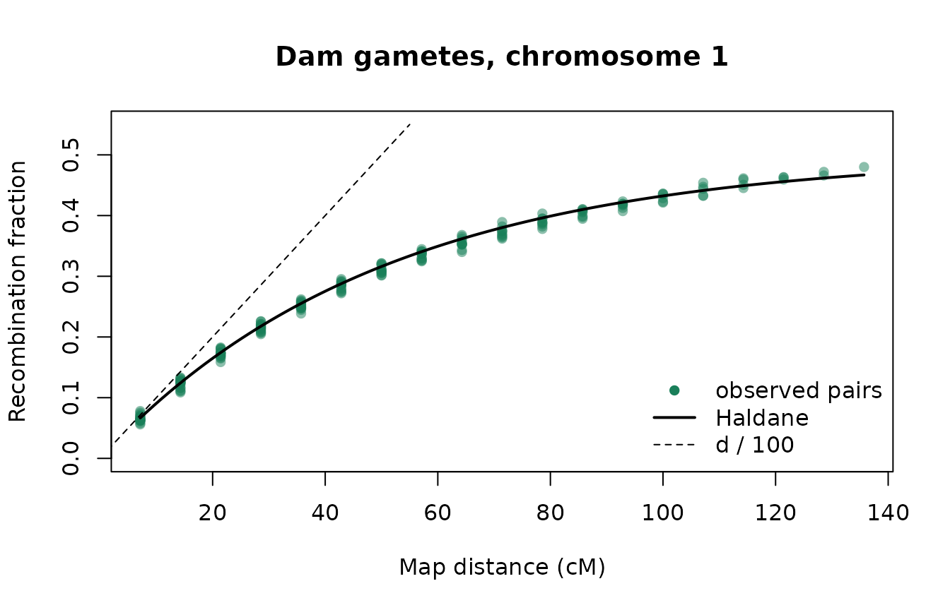

The points sit on the Haldane curve and peel away from the d / 100 line as double crossovers become common. A standardised residual, z = (r_obs - r) / sqrt(r (1 - r) / n), puts every pair on one scale; a correct model gives values within a few units of 0:

z_summary <- function(x) {
  r <- haldane(x$d)
  z <- (x$r_obs - r) / sqrt(r * (1 - r) / x$n)
  c(pairs = nrow(x), max_abs_z = round(max(abs(z)), 2))
}
rbind(
  "dam, chr 1 (1 cM/Mb)"   = z_summary(dam_chr1),
  "sire, chr 1 (1 cM/Mb)"  = z_summary(pair_rates(f2_haps, "1", 1)),
  "dam, chr 2 (0.5 cM/Mb)" = z_summary(pair_rates(f2_haps, "2", 2)),
  "dam, X"                 = z_summary(pair_rates(f2_haps, "3", 2))
)
#>                        pairs max_abs_z
#> dam, chr 1 (1 cM/Mb)     190      1.83
#> sire, chr 1 (1 cM/Mb)    190      2.50
#> dam, chr 2 (0.5 cM/Mb)   190      2.58
#> dam, X                   190      2.52

Crossover counts

The number of crossovers a gamete has on a chromosome should be Poisson with mean L / 100. ind_crossover has one row per crossover; a gamete with none has no row, so the zeros are added back:

xo_counts <- get_table(pop, "ind_crossover") |>
  filter(substr(id_ind, 1, 3) == "F2_", parent_origin == 2, chr_name == "1") |>
  count(id_ind) |>
  collect()
n_xo <- c(xo_counts$n, rep(0L, n_f2 - nrow(xo_counts)))

L1 <- max(map$pos_cM[map$chr_name == "1"])
k  <- 0:max(n_xo)
rbind(observed = tabulate(n_xo + 1L, nbins = length(k)),
      expected = round(n_f2 * dpois(k, L1 / 100), 1)) |>
  `colnames<-`(k)
#>              0     1     2     3    4    5   6
#> observed 364.0 531.0 345.0 168.0 63.0 25.0 4.0
#> expected 359.5 513.5 366.8 174.7 62.4 17.8 4.2
c(mean = mean(n_xo), variance = var(n_xo), expected = L1 / 100)
#>     mean variance expected 
#> 1.417333 1.458805 1.428571

Sex-dependent rules

The chromosome rules change what a parent passes on:

Achiasmy. Chromosome 2 does not recombine in males, so an F1 sire passes one of his two chromosome 2 copies whole: every pair of loci has recombination fraction 0, while the dams’ gametes follow the map.
The X. An F1 male has a single X, from his line B dam. He passes it unchanged to every daughter and nothing to his sons; the F1 females’ X recombines at the map rate (the “dam, X” row above).

sire_chr2 <- pair_rates(f2_haps, "2", 1)
c(max_r_sire_chr2 = max(sire_chr2$r_obs))
#> max_r_sire_chr2 
#>               0

pat_x <- f2_haps |>
  filter(chr_name == "3", parent_origin == 1) |>
  inner_join(get_table(pop, "ind_meta") |> select(id_ind, sex) |> collect(),
             by = "id_ind")
table(offspring_sex = pat_x$sex, line_origin = pat_x$line_origin)
#>              line_origin
#> offspring_sex     B
#>             F 15000

Only daughters carry a paternal X, and it is always line B.

Assumptions and limits

No crossover interference. Crossovers are independent (Haldane). Real meiosis spaces crossovers apart and usually forces at least one per chromosome pair, which the Kosambi map function approximates. The Haldane model therefore slightly overstates double recombinants over short distances. For simulating linkage disequilibrium and selection response this is the standard choice.
The chromosome ends at its last locus. The crossover count uses the last locus’s position, not chr_len_Mb * cM_per_Mb. Alleles are unaffected, but crossover counts read from ind_crossover are those of the mapped segment.
A chromosome at most 3000 cM long. Longer is refused as almost certainly a units error.
Sex- and line-specific maps are honoured by add_offspring(), but define_genome() writes only the default map.

The checks in this article are run, with fixed seeds and larger samples, in the package’s test suite (tests/testthat/test-recombination_rates.R), together with a male-specific map twice the default length.