# The measurement table above, as a matrix. byrow = TRUE fills it the way the
# table reads: across row 1, then across row 2.
Y <- matrix(c(48, 25,
              52, 28,
              41, 22,
              45, 25), nrow = 4, byrow = TRUE)
Y
#>      [,1] [,2]
#> [1,]   48   25
#> [2,]   52   28
#> [3,]   41   22
#> [4,]   45   25

dim(Y)      # rows first, always: 4 by 2
#> [1] 4 2
Y[3, 2]     # row 3, column 2 -- lamb 3's loin depth, 22
#> [1] 22

# One column on its own is a vector. We will use the weights repeatedly, so
# give them a name now.
y <- Y[, 1]
y
#> [1] 48 52 41 451 Matrix Algebra for Animal Breeders
No prerequisites — this is the entry point.
1.1 Why linear algebra?
Figure 1.1 is this chapter on one page. Nothing in it needs to make sense yet — come back to it when you have finished, and use it as a map in the meantime.
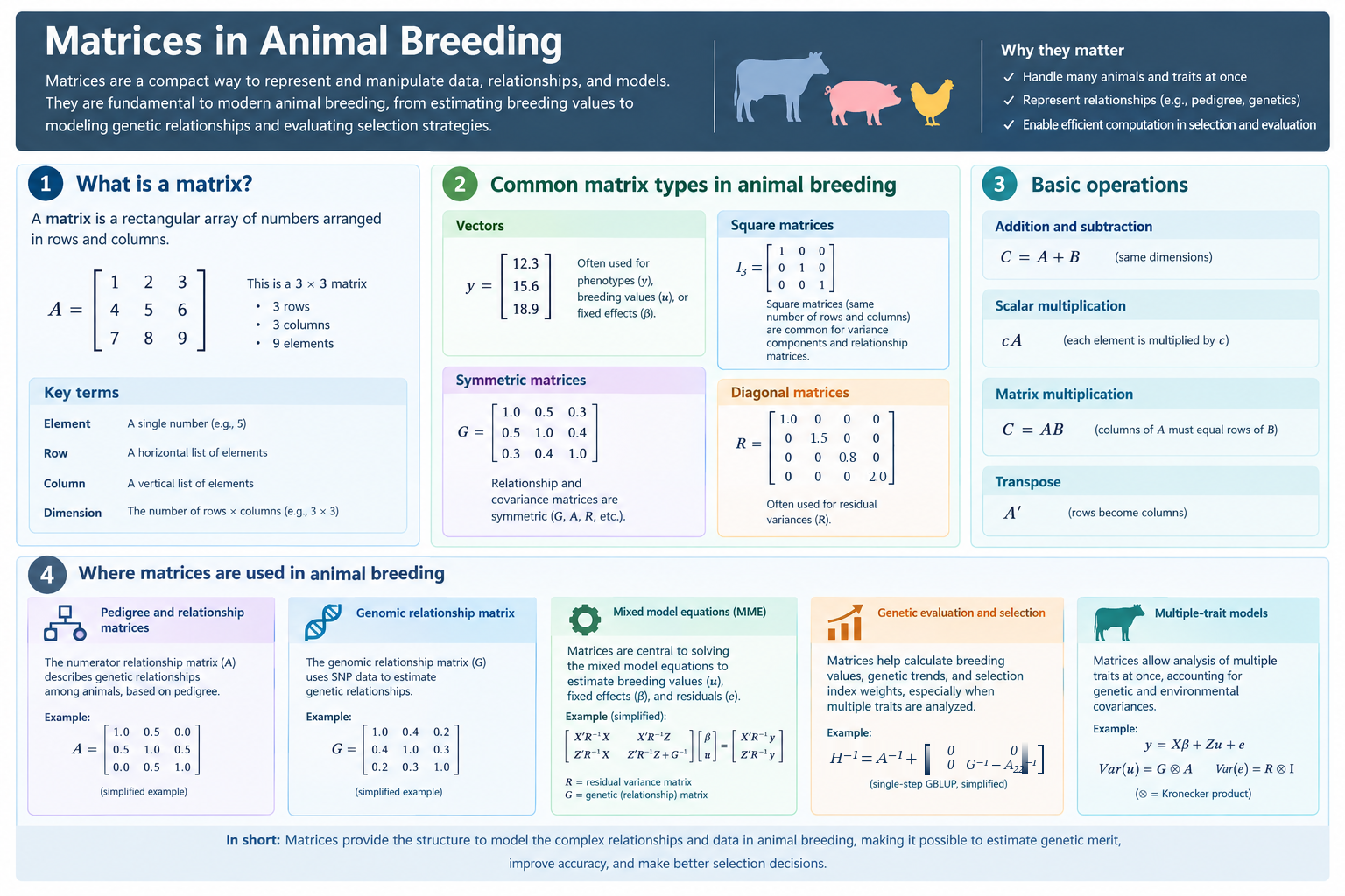
Two entries in the bottom row — the genomic relationship matrix and single-step GBLUP — are outside this book’s scope and belong to the companion volume on genomics. They are in the figure so you can see where the pedigree-based methods you are about to learn eventually lead, not because they are taught here.
1.1.1 What it is
Linear algebra is the mathematics of many quantities at once. Ordinary algebra handles one unknown at a time: solve 4x = 12 and you have x = 3. Animal breeding never asks a question that small. A genetic evaluation asks for the breeding values of every animal in a population simultaneously, because no animal’s value can be worked out without its relatives’ — and those depend back on it. That is not one equation. It is a hundred thousand equations that must all be true at the same time.
Linear algebra is the language for writing down such a system and solving it. It gives you two things ordinary algebra cannot:
- A way of writing that does not grow with the problem. The same four symbols describe four animals or four million. You will see this happen in §1.7.
- Operations on whole collections of numbers at once — an arithmetic where the objects being added and multiplied are entire tables rather than single values.
The word linear is a real restriction and worth knowing about. It means every unknown appears only to the first power, multiplied by a constant and added to the others — no squares, no products of two unknowns, no unknowns inside a logarithm. Most of quantitative genetics is built to stay inside that restriction, because linear systems are the ones we can actually solve at scale. The threshold models of Chapter 14 are what it looks like when a trait refuses to fit, and what has to be done about it.
1.1.2 Where it appears in animal breeding
Almost every quantitative method a breeder uses is linear algebra with a different name on it. The table below is the map: the left column is where you meet the problem, the middle column is what the algebra actually has to do, and the right column is the section of this chapter that teaches it.
| Where it shows up | What the linear algebra does | Taught in |
|---|---|---|
| The animal model (Ch 6) | Build the mixed model equations (Henderson 1975), solve them for every effect at once, and read accuracy off the inverted coefficient matrix | §1.5, §1.9, §1.15 |
| Relationship matrices (Ch 4) | Build A from a pedigree and invert it — the object that makes the animal model practical (Henderson 1976) | §1.9, §1.12 |
| Selection index (Ch 6) | Find the weights that combine an animal’s own record with its relatives’ by solving a linear system, \mathbf{b} = \mathbf{P}^{-1}\mathbf{Ga} (Hazel 1943) | §1.9 |
| Fixed effects and contemporary groups (Ch 2, Ch 5) | Decide which effects can be estimated at all, and which herds can be compared with which | §1.8, §1.10 |
| Multiple traits (Ch 11) | Expand a small trait covariance matrix over every animal in the pedigree | §1.11 |
| Random regression (Ch 12) | Fit a curve per animal from a polynomial basis, and reduce twenty traits to the few dimensions carrying the variation | §1.13 |
| Variance components (Ch 20–22) | Build a likelihood out of quadratic forms, traces, and log-determinants, then differentiate it (Patterson and Thompson 1971) | §1.12, §1.14 |
| Simulation (Ch 11, Ch 22) | Turn independent random draws into correlated breeding values with the right covariance structure | §1.12, §1.15 |
| Solving at scale (Ch 24) | Get an answer when the coefficient matrix has a million rows and cannot be inverted directly | §1.9 |
| Optimal contribution selection | Maximise genetic merit subject to a ceiling on average relationship — a quadratic form \mathbf{x}'\mathbf{Ax} in the contributions | §1.14 · theory in the companion volume on breeding programme design |
| Genomic prediction | Replace A with a relationship matrix built from markers. The surrounding algebra does not change | companion volume on genomics |
Two things are worth noticing about that list before you start.
The same few operations keep reappearing. Multiply, transpose, invert, decompose. Optimal contribution selection and REML look nothing like each other on the page, yet both rest on a quadratic form — the object of §1.14 — and both need the same relationship matrix. Learning an operation once buys you every application of it, which is why this chapter is organised by operation rather than by application.
The last two rows are deliberately out of scope here. Optimal contribution selection belongs to breeding programme design and genomic prediction to genomics; each has a companion volume, and neither is taught in this book. They are in the table because the algebra underneath them is the algebra in this chapter — a student who works through Chapter 1 is equipped for both. ### Why not just run the software?
Every operation in this chapter is one line of R, and nobody computes a national evaluation by hand. So why learn to?
Because much of what goes wrong in a real evaluation is visible in the algebra before it is visible in the results — and sometimes never visible in the results at all. An effect that cannot be estimated still returns a number (§1.10). A genetic correlation of exactly 1 stops REML converging, and the error names a matrix rather than the pair of traits that caused it (§1.13). Two herds with no animals in common produce breeding values that look comparable and are not (Chapter 5). In each case the software is behaving correctly; the person reading the output is the one who has to recognise what happened.
The narrower reason is that Chapter 6 is unreadable without this material. Henderson’s equations are written in matrices, solved with a matrix inverse, and their accuracies read off a matrix diagonal. A student who cannot form \mathbf{X}'\mathbf{X} cannot see what those equations are doing, and is left running software and trusting the output — which is exactly the position the paragraph above says you should not be in.
It is worth knowing how far this transfers, too. Regression, ANOVA, and the general linear model are the same computation as §1.9 with different words attached: lm() in R forms \mathbf{X}'\mathbf{X} and solves it, using the drop-a-level generalized inverse of §1.10.
1.1.3 How to use this chapter
This is a reference. Read it once to see what is here, then come back to whichever section you need — §1.16 maps every section to the chapters that consume it. Every section opens with real numbers and works them before stating any rule, so landing in §1.14 without having read §1.4 still works.
Three small examples carry the whole chapter, and they are reused on purpose: the algebra changes while the animals stay the same, which is the only way to see that it is the algebra doing the work.
1.2 Matrices, vectors, and scalars
Before any operation, the objects themselves. Everything in this chapter is one of three things, and a great deal of confusion later comes from losing track of which.
1.2.1 The objects
Four lambs were measured for two traits — yearling weight in kilograms and loin muscle depth in millimetres:
| Lamb | Yearling weight (kg) | Loin depth (mm) |
|---|---|---|
| 1 | 48 | 25 |
| 2 | 52 | 28 |
| 3 | 41 | 22 |
| 4 | 45 | 25 |
Strip away the headings and what is left is eight numbers in a rectangle, four rows deep and two columns wide:
\mathbf{Y} = \begin{bmatrix} 48 & 25 \\ 52 & 28 \\ 41 & 22 \\ 45 & 25 \end{bmatrix}
That is a matrix, and it is the only object this chapter is really about. Nothing has been modelled, assumed, or estimated. The rectangle is just the data, arranged so that position carries meaning: row 3 is lamb 3, column 2 is loin depth, and the number where they meet — 22 — is lamb 3’s loin depth.
NoteDefinition — Matrix, vector, and scalar
A matrix is a rectangular array of numbers in which position carries meaning. A vector is a matrix with a single column. A scalar is a single number.
Its dimensions are quoted rows first: \mathbf{Y} above is 4 × 2, read “four by two”. The number in row i and column j is called an element and written y_{ij}, again row first, so y_{32} = 22.
Why it matters. These three words are the whole vocabulary of the chapter, and the book uses typography to keep them apart: bold uppercase for a matrix (\mathbf{Y}, \mathbf{X}, \mathbf{A}), bold lowercase for a vector (\mathbf{y}, \mathbf{b}), plain italic for a scalar (\sigma^2_e, \alpha). When you meet \mathbf{Y} and \mathbf{y} in the same equation in Chapter 11, they are different objects and the case is the only thing telling you so.
Take one column of \mathbf{Y} on its own — the four weights — and you have a vector, 4 × 1:
\begin{bmatrix} 48 \\ 52 \\ 41 \\ 45 \end{bmatrix}
This is the shape almost everything in the book arrives in: one row per record, in a fixed order that never changes. That fixed order is what lets a second table — which flock each lamb is in, which sire it is by — line up against it row by row without anyone having to say so.
1.2.2 The one idea underneath all of it
Suppose you wanted a single index combining both traits, counting a kilogram of weight as worth 1 and a millimetre of depth as worth 2. For lamb 1 that is
1(48) + 2(25) = 98
Multiply each quantity by a weighting, add up the results. That operation — and only that operation — is what linear algebra automates.
NoteDefinition — Linear combination
A linear combination of a set of quantities is what you get by multiplying each one by a constant and adding the results: c_1x_1 + c_2x_2 + \cdots + c_nx_n. The constants are called coefficients or weights.
Why it matters. This is the single idea the whole chapter is built from, and recognising it saves you learning the same thing five times. Matrix multiplication (§1.5) is linear combinations performed wholesale. A fitted value \mathbf{Xb} is a linear combination of effects. A selection index is a linear combination of trait records. A breeding value is a linear combination of the information on an animal and its relatives. Every one of them is “multiply by weights, then add” — what changes between them is only where the weights come from.
The same weights applied to every lamb at once, still one multiplication and one addition per term:
1 * Y[, 1] + 2 * Y[, 2]     # 98 for lamb 1, and the other three
#> [1]  98 108  85  95
Section 1.5 replaces that line with a single matrix product. Nothing about the arithmetic changes — only how much of it you have to write down.
1.2.3 Notation
These are conventions, not results. There is nothing to discover — they are names, and you should be handed them rather than led to them.
The book writes bold uppercase for a matrix, bold lowercase for a vector, and plain italic for a scalar, as set out above. Two more pieces of vocabulary before we start operating on them.
A matrix is square when it has as many rows as columns. Only square matrices have determinants, inverses, and eigenvalues, so a good deal of this chapter applies to them alone. Our \mathbf{Y} is 4 × 2 and therefore not square — but \mathbf{Y}'\mathbf{Y} would be, and it is no accident that the products at the centre of every model in this book come out square however many records you have.
The main diagonal of a square matrix runs from its top-left corner to its bottom-right: the elements a_{11}, a_{22}, a_{33}, \ldots, the ones whose row and column index are the same. Almost everything interesting about a square matrix is either on that diagonal or defined relative to it.
1.3 Transpose
The simplest operation there is. It needs nothing but the matrix itself, which is why it comes first.
Write the measurement matrix \mathbf{Y} from §1.2, and then write it again with its rows and columns interchanged:
\mathbf{Y} = \begin{bmatrix} 48 & 25 \\ 52 & 28 \\ 41 & 22 \\ 45 & 25 \end{bmatrix} \qquad \mathbf{Y}' = \begin{bmatrix} 48 & 52 & 41 & 45 \\ 25 & 28 & 22 & 25 \end{bmatrix}
\mathbf{Y} is 4 × 2 and \mathbf{Y}' is 2 × 4. Row 1 of \mathbf{Y} — lamb 1’s two measurements — has become column 1 of \mathbf{Y}'. The entry that sat in row 3, column 2 now sits in row 2, column 3. That is the whole operation, and written out it is simply
y'_{ij} = y_{ji}
The transpose is written \mathbf{Y}' in this book and read “Y prime”; some texts write \mathbf{Y}^{T} for the same thing. Transposing twice puts everything back, so (\mathbf{Y}')' = \mathbf{Y}.
t(Y)                    # 4 x 2 becomes 2 x 4
#>      [,1] [,2] [,3] [,4]
#> [1,]   48   52   41   45
#> [2,]   25   28   22   25
all.equal(t(t(Y)), Y)   # transposing twice returns the original
#> [1] TRUE
A square matrix that is unchanged by transposing is called symmetric: its element in row i, column j equals the one in row j, column i, so it is a mirror image of itself across the diagonal running from top-left to bottom-right.
\begin{bmatrix} 1 & 0.5 \\ 0.5 & 1 \end{bmatrix}
That matters more than it looks. Every relationship matrix and every covariance matrix in this book is symmetric, because the relationship between animal 1 and animal 2 is the same number as the relationship between animal 2 and animal 1. So is \mathbf{X}'\mathbf{X} (§1.7), and so is the whole left-hand side of the mixed model equations in Chapter 6. It is a fact used constantly and almost never announced, and it is worth carrying: whenever you see \mathbf{A}' written for a covariance matrix, it is the same matrix as \mathbf{A}.
1.4 Addition, subtraction, and scalar multiplication
Like the transpose, these three leave every number where it is. Nothing travels; position is preserved. That is exactly what makes them easy, and it is the property matrix multiplication gives up in §1.5.
1.4.1 Addition and subtraction
Matrix addition is element by element, position preserved. Here is the case worth caring about.
For sheep yearling weight (kg) and loin muscle depth (mm), suppose the additive genetic covariance matrix and the residual covariance matrix are
\mathbf{G} = \begin{bmatrix} 36 & 12 \\ 12 & 9 \end{bmatrix} \qquad \mathbf{R} = \begin{bmatrix} 64 & 4 \\ 4 & 16 \end{bmatrix}
Call these Example B. They are the two-trait covariance structure the rest of the chapter returns to.
Adding them position by position — 36 + 64, 12 + 4, 12 + 4, 9 + 16 — gives the phenotypic covariance matrix:
\mathbf{P} = \mathbf{G} + \mathbf{R} = \begin{bmatrix} 100 & 16 \\ 16 & 25 \end{bmatrix}
Everything a breeder quotes comes off these three matrices by division. The phenotypic standard deviations are \sqrt{100} = 10 kg and \sqrt{25} = 5 mm. The heritabilities are the diagonal of \mathbf{G} over the diagonal of \mathbf{P}: 36/100 = 0.36 for weight and 9/25 = 0.36 for depth. The genetic correlation is the off-diagonal of \mathbf{G} over the square root of the product of its diagonals, 12/\sqrt{36 \times 9} = 12/18 = 0.67; the residual correlation is 4/\sqrt{64 \times 16} = 0.125; the phenotypic correlation is 16/(10 \times 5) = 0.32.
G <- matrix(c(36, 12,
              12,  9), nrow = 2)   # additive genetic covariances
R <- matrix(c(64,  4,
               4, 16), nrow = 2)   # residual covariances
P <- G + R                         # phenotypic covariances, element by element
P
#>      [,1] [,2]
#> [1,]  100   16
#> [2,]   16   25

# Heritabilities: the diagonal of G over the diagonal of P. diag() pulls out
# the main diagonal of a square matrix -- the elements defined in section 1.2.
diag(G) / diag(P)
#> [1] 0.36 0.36

# Correlations: an off-diagonal over the root of the product of its diagonals.
G[1, 2] / sqrt(G[1, 1] * G[2, 2])   # genetic,     0.667
#> [1] 0.6666667
R[1, 2] / sqrt(R[1, 1] * R[2, 2])   # residual,    0.125
#> [1] 0.125
P[1, 2] / sqrt(P[1, 1] * P[2, 2])   # phenotypic,  0.32
#> [1] 0.32
Subtraction works the same way, and it is how \mathbf{R} is usually obtained in practice: \mathbf{R} = \mathbf{P} - \mathbf{G}. Addition requires identical dimensions — there is no sensible answer to “what is the 2 × 2 plus the 3 × 3,” and R will refuse.
Scalar multiplication multiplies every element by the same number. It is how the relationship matrix becomes a covariance matrix: \mathbf{G} = \mathbf{A}\sigma^2_a for a single trait, so for two full sibs with \sigma^2_a = 36,
\mathbf{A}\sigma^2_a = \begin{bmatrix} 1 & 0.5 \\ 0.5 & 1 \end{bmatrix} \times 36 = \begin{bmatrix} 36 & 18 \\ 18 & 36 \end{bmatrix}
The variance ratio \alpha = \sigma^2_e / \sigma^2_a is a scalar too, and it is the number that controls how much a mixed model shrinks its predictions. With the values above, \alpha = 64/36 = 1.78.
1.5 Matrix multiplication
Transpose, addition and scalar multiplication all leave the numbers where they are. Multiplication does not, and it is the operation everything else in the book is built on. It is also the one students find hardest, so we are going to do it before naming it.
1.5.1 Two totals
Flock A’s two lambs weigh 48 and 52 kg; flock B’s weigh 41 and 45. We want each flock’s total weight. Here are the records, with a bookkeeping column marking which flock each lamb belongs to. Call that table \mathbf{W}. Nothing is being modelled or estimated — we are adding up weights, and the ones and zeros are only there to say which lamb belongs in which total.
\begin{array}{c|cc|c} & \text{flock A} & \text{flock B} & y \\ \hline \text{lamb 1} & 1 & 0 & 48 \\ \text{lamb 2} & 1 & 0 & 52 \\ \text{lamb 3} & 0 & 1 & 41 \\ \text{lamb 4} & 0 & 1 & 45 \end{array}
Flock A’s total: walk down the flock A column, pair each entry with the weight beside it, multiply, and add.
1(48) + 1(52) + 0(41) + 0(45) = 100
Flock B’s total, the same walk down the other column:
0(48) + 0(52) + 1(41) + 1(45) = 86
Two totals, from two columns, against one list of weights. Write them as a pair:
\begin{bmatrix} 100 \\ 86 \end{bmatrix}
What mattered and what did not. The numbers 48 and 52 were these lambs’ weights — change the weights and the totals change. The number of columns we walked through was the number of flocks, and it fixed how many totals came out: two columns in, two totals out. But the walk itself — take a column, pair it term by term with the list, multiply, add — never changed, and it would not change for 4 lambs or 4 million, for 2 flocks or 200. The one thing the walk needed was that the column and the list be the same length, so the pairing never ran out on either side.
That walk is matrix multiplication. Stand the bookkeeping table on its side so its columns become rows — that is the transpose from §1.3 — and the pair of totals is \mathbf{W}'\mathbf{y}, whose ith element pairs row i of \mathbf{W}' with \mathbf{y} term by term and sums:
(\mathbf{W}'\mathbf{y})_i = \sum_k (\mathbf{W}')_{ik}\, y_k
In general, for \mathbf{A} of size m \times n and \mathbf{B} of size n \times p, the product \mathbf{C} = \mathbf{AB} is m \times p with
c_{ij} = \sum_{k=1}^{n} a_{ik} b_{kj}
Element c_{ij} is row i of the left matrix walked against column j of the right one. The condition for this to work is exactly the one we relied on without saying so: the inner dimensions must match. An m \times n times an n \times p works and gives m \times p; the two n’s meet in the middle and cancel, and what survives is the outside pair.
CautionCheck Yourself
You just multiplied a 2 × 4 by a 4 × 1 and got a 2 × 1. Before reading on: what comes out of a 4 × 2 times a 4 × 1, and why?
Answer. Nothing — it cannot be formed. The inner dimensions are 2 and 4, and they do not match, so the pairing runs out after two terms with two weights left over. Written the other way, \mathbf{W}'\mathbf{y} is 2 × 4 times 4 × 1 and works. This is why the bookkeeping table gets transposed before it meets \mathbf{y}, and not for any deeper reason.
NoteDefinition — Conformable
Two matrices are conformable for an operation when their dimensions permit it. For addition and subtraction that means identical dimensions. For multiplication it means something weaker, which §1.5 arrives at by doing it rather than by declaring it.
Why it matters. Non-conformability is the most common error a student makes in R, and it is the useful kind: the operation stops rather than returning a wrong number. When %*% throws “non-conformable arguments”, it is telling you that the two objects do not line up — usually because a matrix needs transposing, and occasionally because the model itself is wrong.
The special matrices below are named by where they appear in this book, because that is how you will meet them.
# The bookkeeping table of the walk above: one column per flock.
W <- cbind(flockA = c(1, 1, 0, 0),
           flockB = c(0, 0, 1, 1))
W
#>      flockA flockB
#> [1,]      1      0
#> [2,]      1      0
#> [3,]      0      1
#> [4,]      0      1

# Transpose it, then multiply. The two flock totals we worked by hand: 100, 86.
t(W) %*% y
#>        [,1]
#> flockA  100
#> flockB   86

# W'W counts instead of summing: how many lambs are in each flock.
t(W) %*% W
#>        flockA flockB
#> flockA      2      0
#> flockB      0      2
TipIn R —
%*% is multiplication; * is not
A * B in R multiplies element by element and is the Hadamard product of §1.11. Matrix multiplication is A %*% B. The trap is that for two matrices of the same shape, A * B runs without error and returns something plausible-looking, so this fails silently.
Once you have written t(X) %*% X a few times, use crossprod(X) instead — and crossprod(X, y) for \mathbf{X}'\mathbf{y}. They give the same answer and are faster, because they never build \mathbf{X}' at all. There is also tcrossprod(X) for \mathbf{XX}'. The rest of this book uses the crossprod forms.
all.equal(crossprod(W), t(W) %*% W)
#> [1] TRUE
all.equal(crossprod(W, y), t(W) %*% y)
#> [1] TRUE
1.5.2 The rule that catches everyone
Now something you cannot read off the page. Take two 2 × 2 matrices with no symmetry and nothing in common:
\mathbf{A} = \begin{bmatrix} 2 & 1 \\ 0 & 3 \end{bmatrix} \qquad \mathbf{B} = \begin{bmatrix} 1 & 4 \\ 2 & 0 \end{bmatrix}
Multiply them — you now know how — and transpose the result:
\mathbf{AB} = \begin{bmatrix} 4 & 8 \\ 6 & 0 \end{bmatrix} \qquad (\mathbf{AB})' = \begin{bmatrix} 4 & 6 \\ 8 & 0 \end{bmatrix}
There are two obvious candidates for what (\mathbf{AB})' ought to equal. Form both:
\mathbf{A}'\mathbf{B}' = \begin{bmatrix} 2 & 4 \\ 13 & 2 \end{bmatrix} \qquad \mathbf{B}'\mathbf{A}' = \begin{bmatrix} 4 & 6 \\ 8 & 0 \end{bmatrix}
The second one matches. The first is not even close.
What mattered and what did not. The particular entries did not matter — nothing about 2, 1, 0 or 3 made the second candidate win. The dimensions did not matter either; had \mathbf{A} been 3 × 5 and \mathbf{B} 5 × 2, \mathbf{A}'\mathbf{B}' would have been 5 × 3 times 2 × 5 and could not have been formed at all. What mattered is that transposing swaps which index runs along which side, so the two factors have to swap as well for the ends still to meet.
ImportantKey Equation — The reversal rules
(\mathbf{AB})' = \mathbf{B}'\mathbf{A}' \tag{1.1}
In words: transposing a product reverses the order of the factors. Watch for the shape of this rule again later — the reversal is not something special about the transpose.
# matrix() fills COLUMN by column, so read these down the columns, not across.
A <- matrix(c(2, 0,
              1, 3), nrow = 2)
B <- matrix(c(1, 2,
              4, 0), nrow = 2)
A
#>      [,1] [,2]
#> [1,]    2    1
#> [2,]    0    3
B
#>      [,1] [,2]
#> [1,]    1    4
#> [2,]    2    0

t(A %*% B)      # (AB)'
#>      [,1] [,2]
#> [1,]    4    6
#> [2,]    8    0
t(B) %*% t(A)   # B'A' -- the same
#>      [,1] [,2]
#> [1,]    4    6
#> [2,]    8    0
t(A) %*% t(B)   # A'B' -- not the same
#>      [,1] [,2]
#> [1,]    2    4
#> [2,]   13    2
WarningCommon Mistake — assuming AB and BA are the same thing
They are usually not, and often only one of them can even be formed. With the same \mathbf{A} and \mathbf{B}:
\mathbf{AB} = \begin{bmatrix} 4 & 8 \\ 6 & 0 \end{bmatrix} \qquad \mathbf{BA} = \begin{bmatrix} 2 & 13 \\ 4 & 2 \end{bmatrix}
Same two matrices, different products. Matrix multiplication is associative ((\mathbf{AB})\mathbf{C} = \mathbf{A}(\mathbf{BC})) and distributive (\mathbf{A}(\mathbf{B}+\mathbf{C}) = \mathbf{AB} + \mathbf{AC}), so you may re-bracket freely — but you may never reorder. When a derivation in a later chapter moves a matrix across another one, it is doing something, and it is worth checking what.
This is the single most productive source of error in the chapters that follow. When you are assembling the mixed model equations and you need the block above the diagonal, it is \mathbf{X}'\mathbf{Z}, and the block below it is \mathbf{Z}'\mathbf{X} — which is (\mathbf{X}'\mathbf{Z})', not \mathbf{X}'\mathbf{Z} again. Having formed \mathbf{A}'\mathbf{B}' once by hand and watched it come out wrong is worth more than reading the rule three times.
1.6 Special matrices
Some matrices turn up so often that they have names. They are worth meeting after the operations, because most of them are defined by how they behave under those operations rather than by what they look like.
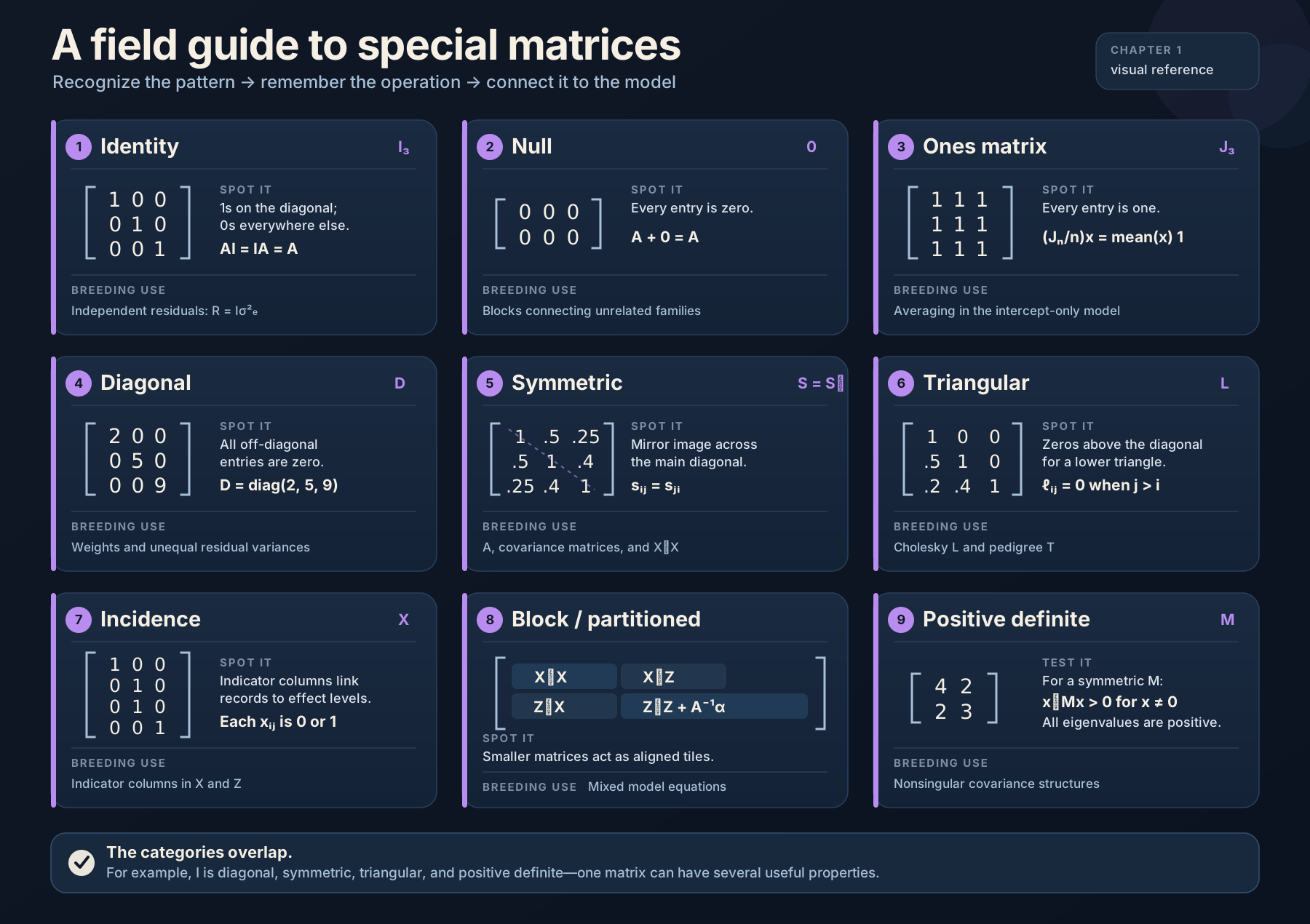
| Matrix | What it is | Where it shows up |
|---|---|---|
| Identity \mathbf{I} | 1s on the diagonal, 0s elsewhere. Multiplying by it changes nothing: \mathbf{AI} = \mathbf{IA} = \mathbf{A} | the residual structure \mathbf{R} = \mathbf{I}\sigma^2_e; the “no relationships” model of Ch 3 |
| Null \mathbf{0} | all zeros | the off-diagonal blocks joining unrelated families |
| \mathbf{J} | all ones | the mean model; \mathbf{J}_n/n as the averaging operator for n entries |
| Diagonal | all off-diagonal entries are zero | weights, unequal residual variances, \mathbf{D} in \mathbf{A} = \mathbf{TDT}' (Ch 4) |
| Symmetric | a_{ij} = a_{ji} | every covariance matrix; \mathbf{X}'\mathbf{X}; the whole MME left-hand side |
| Triangular | zeros above (or below) the diagonal | \mathbf{L} from Cholesky (§1.12); \mathbf{T} from the pedigree (Ch 4) |
| Incidence | 0/1 indicators link records to effect levels | indicator columns in \mathbf{X} and \mathbf{Z} — almost entirely zeros, which is why Ch 24 exists |
| Block / partitioned | built from smaller matrices as tiles | the MME itself (Ch 6) |
| Positive definite | for symmetric \mathbf{M}, \mathbf{x}'\mathbf{Mx} > 0 for every nonzero \mathbf{x} — see §1.13 | nonsingular covariance structures; Cholesky factorisation and inversion |
diag(3)                        # the identity, 3 x 3
#>      [,1] [,2] [,3]
#> [1,]    1    0    0
#> [2,]    0    1    0
#> [3,]    0    0    1
diag(c(2, 5, 9))               # a diagonal matrix from a vector
#>      [,1] [,2] [,3]
#> [1,]    2    0    0
#> [2,]    0    5    0
#> [3,]    0    0    9
matrix(1, nrow = 2, ncol = 3)  # J, all ones, 2 x 3
#>      [,1] [,2] [,3]
#> [1,]    1    1    1
#> [2,]    1    1    1

# Y is the measurement matrix from section 1.2.
nrow(Y)
#> [1] 4
ncol(Y)
#> [1] 2
t(Y)                           # not square: transposing turns 4 x 2 into 2 x 4
#>      [,1] [,2] [,3] [,4]
#> [1,]   48   52   41   45
#> [2,]   25   28   22   25

# A matrix that is mostly zeros, stored sparsely: only the positions of the
# non-zeros are kept, and a dot is printed wherever a zero would be.
Matrix(diag(4), sparse = TRUE)
#> 4 x 4 diagonal matrix of class "ddiMatrix"
#>      [,1] [,2] [,3] [,4]
#> [1,]    1    .    .    .
#> [2,]    .    1    .    .
#> [3,]    .    .    1    .
#> [4,]    .    .    .    1
NoteBeyond This Book — how X is really stored
The incidence matrices \mathbf{X} and \mathbf{Z} in the table above are the reason this matters. The \mathbf{X} built in §1.7 is 4 × 2 and almost half zeros. In a national evaluation it is millions of rows by tens of thousands of columns and more than 99.99% zeros, and no one ever writes it out. Sparse storage — keeping only the positions of the non-zeros — is what makes such a matrix fit in memory at all, and it changes how every operation in this chapter is actually performed. Chapter 24 shows why dense methods fail at that scale; the mechanics of sparse storage and factorisation belong to the companion volume on large-scale computation.
One more piece of notation before we start: \mathbf{X}' — read “X transpose”, or more often just “X prime” — is the subject of §1.3. Some texts write \mathbf{X}^{T} for the same thing.
1.7 Why matrices: one model, many animals
Four lambs were weighed at a year old. Two are from flock A, two from flock B.
| Lamb | Flock | Yearling weight (kg) |
|---|---|---|
| 1 | A | 48 |
| 2 | A | 52 |
| 3 | B | 41 |
| 4 | B | 45 |
We think each lamb’s weight is a flock level plus whatever is left over for that individual. Written one lamb at a time, that is four separate equations. Take flock B as the baseline and let b_1 be flock B’s level and b_2 be however much flock A runs above it:
\begin{aligned} 48 &= b_1 + b_2 + e_1 \\ 52 &= b_1 + b_2 + e_2 \\ 41 &= b_1 \phantom{{}+ b_2} + e_3 \\ 45 &= b_1 \phantom{{}+ b_2} + e_4 \end{aligned}
Every equation has the same two unknowns. What differs between them is only which unknowns appear — a 1 or a 0 in front of each. Pull those coefficients out and write them as a table, one row per lamb, one column per unknown:
\begin{bmatrix} 48 \\ 52 \\ 41 \\ 45 \end{bmatrix} = \begin{bmatrix} 1 & 1 \\ 1 & 1 \\ 1 & 0 \\ 1 & 0 \end{bmatrix} \begin{bmatrix} b_1 \\ b_2 \end{bmatrix} + \begin{bmatrix} e_1 \\ e_2 \\ e_3 \\ e_4 \end{bmatrix}
Four rows, one per record. Two columns, one per thing being estimated: the first column is all ones because every lamb has flock B’s baseline in it, and the second column is 1 exactly when the lamb is in flock A. Call the list of weights \mathbf{y}, the table of ones and zeros \mathbf{X}, the two unknowns \mathbf{b}, and the leftovers \mathbf{e}:
\mathbf{y} = \mathbf{Xb} + \mathbf{e}
Nothing has been gained yet — those are the same four equations with the arithmetic hidden. What has been gained is that the statement no longer mentions four. Add a fifth lamb and \mathbf{y} gets a fifth entry and \mathbf{X} a fifth row; the equation is unchanged. Add 40,000 lambs and it is still unchanged. That invariance is the whole reason this book is written in matrices: the model statement stops depending on how many animals you have, and by Chapter 6 the same four symbols will carry 100,000 pigs without a character of difference.
lambs <- data.frame(lamb  = 1:4,
                    flock = c("A", "A", "B", "B"),
                    wt    = c(48, 52, 41, 45))
lambs| lamb | flock | wt |
|---|---|---|
| 1 | A | 48 |
| 2 | A | 52 |
| 3 | B | 41 |
| 4 | B | 45 |
# y is just the column of weights.
y <- lambs$wt
y
#> [1] 48 52 41 45

# X, built exactly as it is written on the page: a column of ones for flock B's
# baseline, then a 1 wherever the lamb is in flock A.
baseline <- c(1, 1, 1, 1)
flockA   <- c(1, 1, 0, 0)
X <- cbind(baseline, flockA)
X
#>      baseline flockA
#> [1,]        1      1
#> [2,]        1      1
#> [3,]        1      0
#> [4,]        1      0
With \mathbf{X} and \mathbf{y} in hand, the two products of §1.5 finally have their book meanings:
crossprod(X)        # X'X -- the table of counts
#>          baseline flockA
#> baseline        4      2
#> flockA          2      2
crossprod(X, y)     # X'y -- the table of sums
#>          [,1]
#> baseline  186
#> flockA    100

# Xb hands each record its fitted value. b is solved for in §1.9.
b_hat <- c(43, 7)
X %*% b_hat
#>      [,1]
#> [1,]   50
#> [2,]   50
#> [3,]   43
#> [4,]   43
R will also build \mathbf{X} for you from the data frame. That is what you will use in practice, but it is worth seeing only after you have built one by hand, because the function chooses the parameterisation and you need to be able to check which one it chose.
# The same X, from a formula. Listing flock B first makes it the baseline,
# which is the parameterisation we wrote out above.
lambs$flock <- factor(lambs$flock, levels = c("B", "A"))
X_auto <- model.matrix(~ flock, data = lambs)
X_auto
#>   (Intercept) flockA
#> 1           1      1
#> 2           1      1
#> 3           1      0
#> 4           1      0
#> attr(,"assign")
#> [1] 0 1
#> attr(,"contrasts")
#> attr(,"contrasts")$flock
#> [1] "contr.treatment"

# Two cosmetic differences from the X we built by hand: the first column is
# called "(Intercept)" rather than "baseline", and model.matrix() attaches
# bookkeeping attributes of its own. Ignore both -- the numbers are identical.
all.equal(X, X_auto, check.attributes = FALSE)
#> [1] TRUE
1.7.1 X′X counts and X′y sums
Now form \mathbf{X}'\mathbf{X} for the \mathbf{X} just built — the one whose first column is all ones and whose second column flags flock A — and form \mathbf{X}'\mathbf{X} from it. Row 1 of \mathbf{X}' against column 1 of \mathbf{X} is 1(1) + 1(1) + 1(1) + 1(1) = 4. Row 1 against column 2 is 1(1) + 1(1) + 1(0) + 1(0) = 2. Row 2 against column 2 is 1(1) + 1(1) + 0(0) + 0(0) = 2.
\mathbf{X}'\mathbf{X} = \begin{bmatrix} 4 & 2 \\ 2 & 2 \end{bmatrix} \qquad \mathbf{X}'\mathbf{y} = \begin{bmatrix} 186 \\ 100 \end{bmatrix}
Look at what those four numbers are. Every element of \mathbf{X} is a 0 or a 1, so multiplying two of them together gives 1 only when both are 1 — and summing the products just counts the rows where both columns had a 1.
- \mathbf{X}'\mathbf{X} is a table of counts. The 4 is the number of records. The bottom-right 2 is the number of records in flock A. The off-diagonal 2 counts the records that have both a baseline and a flock A indicator — also 2, because every flock A record has both.
- \mathbf{X}'\mathbf{y} is a table of sums. 186 is the grand total of all four weights; 100 is the flock A total we computed above.
These are not facts stated about \mathbf{X}'\mathbf{X} after the fact. They are the reason it gets built. Every left-hand side you will meet in this book is a table of counts with variance ratios added to some of its diagonal, and every right-hand side is a table of sums. A student who owns this reads Chapter 6’s mixed model equations without effort.
Two more products worth naming while we are here. \mathbf{Xb} hands each record its fitted value — with the solution we reach in §1.9, \mathbf{b} = (43, 7)', it gives (50, 50, 43, 43)', flock A’s lambs getting 43 + 7 and flock B’s getting 43. And \mathbf{Zu}, which arrives in Chapter 3, hands each record its own animal’s breeding value in exactly the same way.
1.8 Rank, singularity, and the determinant
The parameterisation in §1.7 was a choice. A more natural-looking one gives every flock its own column and keeps the baseline as well:
\mathbf{X}_3 = \begin{bmatrix} 1 & 1 & 0 \\ 1 & 1 & 0 \\ 1 & 0 & 1 \\ 1 & 0 & 1 \end{bmatrix}
Three columns: a baseline, a flock A indicator, a flock B indicator. Look at them. The second column plus the third column equals the first, in every row. The third column carries no information the other two lack — knowing a lamb is not in flock A already tells you it is in flock B.
Columns that can be built from other columns are linearly dependent, and \mathbf{X}_3 has three columns of which only two carry independent information. Build it and check the claim directly — column 2 plus column 3 really is column 1:
X3 <- cbind(baseline = 1,
            flockA   = c(1, 1, 0, 0),
            flockB   = c(0, 0, 1, 1))
X3
#>      baseline flockA flockB
#> [1,]        1      1      0
#> [2,]        1      1      0
#> [3,]        1      0      1
#> [4,]        1      0      1

X3[, "flockA"] + X3[, "flockB"]      # equals the baseline column, every row
#> [1] 1 1 1 1
all.equal(X3[, "flockA"] + X3[, "flockB"], X3[, "baseline"],
          check.attributes = FALSE)
#> [1] TRUE
R will tell you the rank directly. qr() factorises the matrix and its $rank component counts the independent columns:
qr(X3)$rank        # 2 -- not 3, even though there are three columns
#> [1] 2
ncol(X3)           # 3 columns, so X3 is rank deficient
#> [1] 3

qr(X)$rank         # the two-column X of section 1.7 is full rank
#> [1] 2
ncol(X)
#> [1] 2
Counting columns is only half the story. Transpose \mathbf{X}_3 so that it is 3 \times 4 — three rows, four columns — and ask for the rank again:
t(X3)
#>          [,1] [,2] [,3] [,4]
#> baseline    1    1    1    1
#> flockA      1    1    0    0
#> flockB      0    0    1    1
qr(t(X3))$rank     # still 2
#> [1] 2
The rank did not change, and it could not have reached 4: a matrix with three rows has at most three independent rows, and the number of independent rows always equals the number of independent columns. So the rank of any matrix is capped by its smaller dimension. For a tall design matrix with more records than effects, that cap is the number of columns, which is why the check above compared qr(X3)$rank with ncol(X3). For a wide matrix with more columns than rows the cap is the number of rows — a genotype matrix with 10 animals and 50,000 markers has rank at most 10, however many markers it carries.
NoteDefinition — Linear dependence and rank
A set of columns is linearly dependent when at least one of them can be written as a linear combination (§1.1) of the others — it adds no information the rest do not already carry. Columns that cannot be are linearly independent.
The rank of a matrix is the number of linearly independent columns it has, which is always the same as the number of linearly independent rows. Rank therefore cannot exceed the smaller of the two dimensions: for an n \times p matrix, \text{rank} \le \min(n, p). A matrix whose rank reaches that bound is full rank; one whose rank is smaller is rank deficient. For a tall matrix (n > p), like every design matrix in this book, full rank means rank = p — every column independent. \mathbf{X}_3 is 4 \times 3 with rank 2, so it is rank deficient.
Why it matters. Rank is what decides whether a model’s effects can be estimated at all. In animal breeding the answer is routinely no, and rank deficiency is normal rather than exceptional — every model with a mean and a contemporary group effect has it. Chapter 2 is largely about what to do next, and §1.10 gives the tool.
Form \mathbf{X}_3'\mathbf{X}_3 and the dependence is inherited:
\mathbf{X}_3'\mathbf{X}_3 = \begin{bmatrix} 4 & 2 & 2 \\ 2 & 2 & 0 \\ 2 & 0 & 2 \end{bmatrix}
Again column 2 plus column 3 equals column 1 — the dependence has been inherited:
XtX3 <- crossprod(X3)
XtX3
#>          baseline flockA flockB
#> baseline        4      2      2
#> flockA          2      2      0
#> flockB          2      0      2

XtX3[, 2] + XtX3[, 3]     # still equals column 1
#> baseline   flockA   flockB
#>        4        2        2
qr(XtX3)$rank             # 2, in a 3 x 3 matrix
#> [1] 2
NoteDefinition — Singular matrix
A square matrix is singular when its columns are linearly dependent — equivalently, when its rank is less than its dimension, and when its determinant is zero. Those three statements say the same thing about the same matrix. A square matrix that is not singular is non-singular, or full rank.
A fourth equivalent statement is that a singular matrix has no inverse; §1.9 defines the inverse and shows why the two ideas are the same one.
The practical meaning is that the system of equations the matrix defines has no unique solution. Here you could add any constant to the baseline and subtract it from both flock effects without changing a single fitted value, so there is no single right answer to report.
Why it matters. This is the word your software will use when it refuses to fit a model, and it is worth being able to translate it into “two of the things I asked for cannot be told apart from each other”. The response is not to give up: §1.10 solves the system anyway and tells you which quantities survive. In Chapter 6 the animal block of the mixed model equations is deliberately made non-singular by adding \mathbf{A}^{-1}\alpha to it, which is why the animal model can return a breeding value even for an animal with no record of its own.
1.8.1 Where this material comes from
Rank, linear dependence and the determinant are nineteenth-century mathematics with no single originating paper, so nothing is cited for them above. What does have a literature is the question this section leads into: what to do with a model whose \mathbf{X} is not full rank.
Two results settle it, and both arrived surprisingly late. R. C. Bose gave the definition of an estimable function in the 1940s. Penrose (Penrose 1955) defined the generalized inverse for arbitrary matrices, and Rao (Rao 1962) showed what it does for least squares when the normal equations are singular.
Those dates are worth pausing on, because they fall after Henderson had begun the work this book teaches. Searle — who took his doctorate in animal breeding under Henderson at Cornell — put it plainly in a later interview (Wells 2009): his group had “not kept up with the concept of estimability propounded by R. C. Bose”, nor were they “aware of Penrose’s (1955) generalized inverse matrix which, as Rao (1962) demonstrated, clarified the whole business of solving least squares equations which are so often not of full rank.”
§1.10 is that clarification, and Chapter 2 makes estimability precise.
This is the normal case in animal breeding, not the exceptional one. A contemporary group effect plus an overall mean is exactly the structure above. So is a sex effect with a mean, and a breed effect with a mean. Chapter 2 is largely about what to do with it, and the answer — §1.10 — is not to prevent it but to solve it anyway and be careful about which quantities you then quote.
1.8.2 The determinant
The determinant is a single number computed from a square matrix, written |\mathbf{A}| or \det(\mathbf{A}). For a 2 × 2 it is the difference of the two diagonal products:
\det \begin{bmatrix} a & b \\ c & d \end{bmatrix} = ad - bc
For the full-rank \mathbf{X}'\mathbf{X} of §1.5, \det = (4)(2) - (2)(2) = 4. For a matrix with a redundant column the determinant is 0 — the 3 × 3 above has \det = 0, and so does the 2 × 2 \begin{bmatrix} 100 & 100 \\ 100 & 100 \end{bmatrix}, whose determinant is 100(100) - 100(100) = 0.
det() does all three:
XtX <- crossprod(X)
XtX
#>          baseline flockA
#> baseline        4      2
#> flockA          2      2
(XtX[1, 1] * XtX[2, 2]) - (XtX[1, 2] * XtX[2, 1])   # ad - bc, by hand
#> [1] 4
det(XtX)                                            # the same, 4
#> [1] 4

det(XtX3)          # 0 -- the rank-deficient one
#> [1] 0
Do not memorise the general formula; you will never compute a determinant larger than 3 × 3 by hand, and R does it in one call. Memorise the meaning instead, in its two forms:
- For a design matrix, \det(\mathbf{X}'\mathbf{X}) = 0 means a column is redundant and the effects are not separately estimable.
- For a covariance matrix, \det(\mathbf{G}) = 0 means a genetic correlation of exactly \pm 1 — one trait carries no information the other lacks. The matrix \begin{bmatrix} 100 & 100 \\ 100 & 100 \end{bmatrix} says two traits with \sigma^2_a = 100 each and r_g = 1: genetically, the same trait measured twice. REML will not converge on such a matrix, and Chapter 21 explains why.
Here is that covariance matrix — two traits with \sigma^2_a = 100 each and a genetic correlation of exactly 1:
Gsing <- matrix(c(100, 100,
                  100, 100), nrow = 2)
Gsing
#>      [,1] [,2]
#> [1,]  100  100
#> [2,]  100  100

det(Gsing)          # 0
#> [1] 0
qr(Gsing)$rank      # 1, in a 2 x 2 matrix
#> [1] 1

# The genetic correlation this matrix implies:
Gsing[1, 2] / sqrt(Gsing[1, 1] * Gsing[2, 2])   # exactly 1
#> [1] 1
And this is what R does when you ask it to invert one. solve() computes an inverse — §1.9 is where that is explained — and here it is deliberately being asked for one that does not exist:
solve(Gsing)
#> Error in `solve.default()`:
#> ! Lapack routine dgesv: system is exactly singular: U[2,2] = 0
That message is the one to recognise. “System is exactly singular” is R telling you a column of your matrix is redundant. When it appears in a real analysis it almost always means two effects in the model cannot be told apart from each other — not that anything is broken.
1.8.3 Almost singular: the condition number
Singularity is a yes-or-no property, and the determinant tests it. But a matrix can be non-singular and still behave almost as badly as a singular one. Take the covariance matrix above and lower the genetic correlation from exactly 1 to 0.999:
\mathbf{G} = \begin{bmatrix} 100 & 99.9 \\ 99.9 & 100 \end{bmatrix}, \qquad \det(\mathbf{G}) = 100(100) - 99.9(99.9) = 10000 - 9980.01 = 19.99
Not zero. The columns are independent, the rank is 2, and R will invert it without complaint. Now use it to solve a system, twice, with two right-hand sides that differ by one per cent in one element. First \mathbf{Gx} = (1, 1)':
\begin{aligned} 100x_1 + 99.9x_2 &= 1 \\ 99.9x_1 + 100x_2 &= 1 \end{aligned}
The two equations are symmetric, so x_1 = x_2 and 199.9x_1 = 1, giving x_1 = x_2 = 0.0050. Then \mathbf{Gx} = (1, 1.01)':
\begin{aligned} 100x_1 + 99.9x_2 &= 1 \\ 99.9x_1 + 100x_2 &= 1.01 \end{aligned}
Subtracting the second equation from the first gives 0.1x_1 - 0.1x_2 = -0.01, so x_1 - x_2 = -0.1. Adding them gives 199.9(x_1 + x_2) = 2.01, so x_1 + x_2 = 0.01006. Together, x_1 = -0.0450 and x_2 = 0.0550.
Look at what happened. The right-hand side moved by 0.01 in one element — under one per cent of its length. The solution went from (0.0050, 0.0050)' to (-0.0450, 0.0550)': ten times larger, and one element changed sign. A change of 0.7% in the input became a change of 1000% in the output, an amplification of about 1400. Here it is in R — solve(G, b) solves \mathbf{Gx} = \mathbf{b} directly, and §1.9 says more about it:
G <- matrix(c(100, 99.9,
              99.9, 100), nrow = 2)
det(G)                          # 19.99 -- not zero, so not singular
#> [1] 19.99

x  <- solve(G, c(1, 1))         # the first system
x2 <- solve(G, c(1, 1.01))      # the second, 1% different in one element
x
#> [1] 0.005002501 0.005002501
x2
#> [1] -0.04497249  0.05502751
The amplification is not an accident of these two right-hand sides. Every matrix has a worst-case amplification factor, its condition number, and R computes it with kappa(). The reciprocal, rcond(), is what solve() checks before it agrees to proceed:
kappa(G, exact = TRUE)          # 1999: input error can be amplified up to ~2000 times
#> [1] 1999
rcond(G)                        # 1/1999, the reciprocal that solve() inspects
#> [1] 0.0005002501

kappa(XtX, exact = TRUE)        # the full-rank X'X of section 1.5, for comparison
#> [1] 6.854102
The 1400-fold amplification observed above sits below the bound of 1999, as it must. The \mathbf{X}'\mathbf{X} of §1.5 has a condition number of about 6: a well-behaved matrix, whose solutions move roughly as much as its inputs do.
Push the correlation closer still to 1 and the determinant is still not zero — but solve() refuses anyway, with a different message from the one above:
Gnear <- matrix(c(100, 100 - 1e-14,
                  100 - 1e-14, 100), nrow = 2)
det(Gnear)                      # tiny, but not zero
#> [1] 2.842171e-12
solve(Gnear)
#> Error in `solve.default()`:
#> ! system is computationally singular: reciprocal condition number = 7.10543e-17
“Computationally singular” is the second message to recognise. It means the matrix is non-singular in exact arithmetic but its condition number is so large — here about 10^{16} — that in the sixteen or so decimal digits a computer carries, the inverse would be pure rounding error. solve() declines rather than return nonsense.
NoteDefinition — Condition number
The condition number of a matrix, written \kappa(\mathbf{A}), is the largest factor by which a relative change in the right-hand side \mathbf{b} can be amplified into a relative change in the solution \mathbf{x} of \mathbf{Ax} = \mathbf{b}. It is 1 for the identity matrix, infinite for a singular matrix, and a matrix with a large condition number is ill-conditioned. For the symmetric matrices in this book it equals the largest eigenvalue divided by the smallest — §1.13 shows this for \mathbf{G}, whose eigenvalues are 199.9 and 0.1.
A working rule: a condition number of 10^k costs about k decimal digits of accuracy in the solution. Double-precision arithmetic carries about 16, so \kappa \approx 10^{16} is indistinguishable from singular, which is exactly what “computationally singular” reports.
Why it matters. The determinant tells you whether a system has a unique solution; the condition number tells you whether that solution means anything. An ill-conditioned matrix has a unique solution that rounding error in the data can move anywhere. In this book it appears when two traits have a genetic correlation near \pm 1 (Chapter 11), when two fixed effects are nearly but not quite confounded — a contemporary group almost every one of whose animals share a sire (Chapter 5), and when REML wanders toward the boundary of the parameter space (Chapter 21). It also sets the speed of the iterative solvers in Chapter 24: they converge in a number of iterations that grows with \kappa, which is why they precondition the equations before starting.
1.8.4 Improving the condition of a matrix
A condition number is a property of the matrix you built, and most of the time you can build a better one. The commonest cause of ill-conditioning in a design matrix is not a subtle near-dependence between effects — it is a covariate that was never centred. Take four lambs weighed at 180, 182, 185 and 187 days of age and fit a mean plus a linear effect of age:
\mathbf{X} = \begin{bmatrix} 1 & 180 \\ 1 & 182 \\ 1 & 185 \\ 1 & 187 \end{bmatrix}, \qquad \mathbf{X}'\mathbf{X} = \begin{bmatrix} 4 & 734 \\ 734 & 134718 \end{bmatrix}
Nothing is redundant here: the age column is not a multiple of the column of ones. But it is nearly one. Every age is within 4 days of 183.5, so the second column is 183.5 times the first plus a small wobble, and the two columns point in almost the same direction. The determinant is 4(134718) - 734^2 = 538872 - 538756 = 116 — small next to the entries of the matrix, and the condition number is enormous:
age <- c(180, 182, 185, 187)
X_age <- cbind(1, age)
XtX_age <- crossprod(X_age)
XtX_age
#>            age
#>       4    734
#> age 734 134718
kappa(XtX_age, exact = TRUE)      # about 160 million
#> [1] 156465664
Now subtract the mean age, 183.5, from each age before building \mathbf{X}. The model is the same — the intercept now means “the fitted weight at 183.5 days” instead of “at 0 days”, and the slope is unchanged — but the two columns are now at right angles, because the deviations sum to zero:
\mathbf{X}_c = \begin{bmatrix} 1 & -3.5 \\ 1 & -1.5 \\ 1 & 1.5 \\ 1 & 3.5 \end{bmatrix}, \qquad \mathbf{X}_c'\mathbf{X}_c = \begin{bmatrix} 4 & 0 \\ 0 & 29 \end{bmatrix}
age_c <- age - mean(age)          # deviations: -3.5, -1.5, 1.5, 3.5
X_c <- cbind(1, age_c)
XtX_c <- crossprod(X_c)
XtX_c
#>         age_c
#>       4     0
#> age_c 0    29
kappa(XtX_c, exact = TRUE)        # 7.25
#> [1] 7.25
From 160 million to 7.25, without changing the fitted values by a single gram. That is the first thing to try, and Chapter 5 makes centring covariates a routine step of data preparation. The other tools are variations on the same theme, each of which returns in a later chapter:
- Scale the columns so their diagonals are comparable — divide each column of \mathbf{X} by its standard deviation, or equivalently pre- and post-multiply \mathbf{X}'\mathbf{X} by \mathbf{D}^{-1/2} where \mathbf{D} holds its diagonal. This is what the iterative solvers of Chapter 24 do when they precondition, and on its own it takes the uncentred matrix above from 160 million to about 18,000; centring does the rest.
- Remove the near-dependence rather than living with it: merge two contemporary groups that share almost all their animals, or drop a covariate that is nearly a linear function of another. Chapter 5 is where this happens. A near-singular \mathbf{X} is usually telling you the data cannot support two separate effects, and the honest fix is to ask for one.
- Add to the diagonal. Adding a constant to every diagonal element of a symmetric matrix adds it to every eigenvalue, which raises the smallest one proportionally far more than the largest. For \mathbf{G} above, adding 1 to each diagonal takes \kappa from 1999 to 183. This cannot be done casually to \mathbf{X}'\mathbf{X} — it changes the estimates — but it is exactly what the mixed model equations of Chapter 3 do to the random-effects block, where the added term \mathbf{A}^{-1}\alpha is what makes an otherwise singular \mathbf{Z}'\mathbf{Z} invertible. For an estimated genetic covariance matrix, the principled version is bending (Hayes and Hill 1981): shrink the eigenvalues toward their mean, leaving the eigenvectors alone, until the matrix is positive definite and usably conditioned. Chapter 21 returns to it.
D_half <- diag(1 / sqrt(diag(XtX_age)))          # 1/sqrt of the diagonal
kappa(D_half %*% XtX_age %*% D_half, exact = TRUE)   # scaling alone: ~18,000
#> [1] 18579.79

kappa(G + diag(1, 2), exact = TRUE)                  # 1 on the diagonal of G: 1999 -> 183
#> [1] 182.6364
1.9 Inversion, solving, and partitioned matrices
1.9.1 Finding an inverse without a formula
The inverse of a square matrix \mathbf{A} is the matrix \mathbf{A}^{-1} for which \mathbf{AA}^{-1} = \mathbf{A}^{-1}\mathbf{A} = \mathbf{I}. That definition is not just a description — it is enough to find one.
Take \mathbf{X}'\mathbf{X} = \begin{bmatrix} 4 & 2 \\ 2 & 2 \end{bmatrix} from §1.5, call the unknown inverse \begin{bmatrix} w & x \\ z & v \end{bmatrix}, and demand that the product be the identity:
\begin{bmatrix} 4 & 2 \\ 2 & 2 \end{bmatrix} \begin{bmatrix} w & x \\ z & v \end{bmatrix} = \begin{bmatrix} 1 & 0 \\ 0 & 1 \end{bmatrix}
Multiplying out, one element of the identity at a time, gives four equations in four unknowns:
\begin{aligned} 4w + 2z &= 1 \qquad & 4x + 2v &= 0 \\ 2w + 2z &= 0 \qquad & 2x + 2v &= 1 \end{aligned}
The left pair: subtract the second from the first to get 2w = 1, so w = 0.5, and then z = -0.5. The right pair: subtract to get 2x = -1, so x = -0.5, and then v = 1.
(\mathbf{X}'\mathbf{X})^{-1} = \begin{bmatrix} 0.5 & -0.5 \\ -0.5 & 1 \end{bmatrix}
Multiply back to confirm: \begin{bmatrix} 4 & 2 \\ 2 & 2 \end{bmatrix}\begin{bmatrix} 0.5 & -0.5 \\ -0.5 & 1 \end{bmatrix} = \begin{bmatrix} 1 & 0 \\ 0 & 1 \end{bmatrix}. It is the inverse.
What mattered and what did not. The particular entries 4, 2, 2, 2 set the answers, obviously. But look at the shape of what came out. Every entry is something over 4 — and 4 is \det(\mathbf{X}'\mathbf{X}), computed in §1.8. The two diagonal entries traded places (the 4 and the 2 in the original became a 2/4 and a 4/4). The two off-diagonal entries kept their positions but changed sign. None of that depended on the numbers; solve those four equations with any a, b, c, d and the same three things happen.
ImportantKey Equation — The inverse of a 2 × 2
\begin{bmatrix} a & b \\ c & d \end{bmatrix}^{-1} = \frac{1}{ad - bc}\begin{bmatrix} d & -b \\ -c & a \end{bmatrix} \tag{1.2}
In words: swap the diagonal entries, flip the sign of the off-diagonal ones, and divide everything by the determinant. In general \mathbf{A}^{-1} = \operatorname{adj}(\mathbf{A})/\det(\mathbf{A}), of which this is the 2 × 2 case — the only one you will ever compute by hand.
The division makes §1.8 obvious in hindsight. If \det(\mathbf{A}) = 0 there is nothing to divide by, and the inverse does not exist. “Singular” and “not invertible” are the same statement.
NoteDefinition — Inverse
The inverse of a square matrix \mathbf{A}, written \mathbf{A}^{-1}, is the matrix for which \mathbf{AA}^{-1} = \mathbf{A}^{-1}\mathbf{A} = \mathbf{I}. It is the matrix equivalent of a reciprocal, and it exists only when \mathbf{A} is non-singular.
Why it matters. Inverting is how a matrix equation gets solved, and \mathbf{A}^{-1} — the inverse of the relationship matrix — is the single object that makes the animal model practical (Chapter 4). Note the two cautions that follow: do not compute an inverse merely to solve a system (below), and remember that the inverse of a covariance matrix is a precision matrix, which is why relationships enter Henderson’s equations as information rather than as covariance.
1.9.2 Three inverses worth recognising
The inverse of a diagonal matrix is the diagonal matrix of reciprocals — nothing else to do:
\begin{bmatrix} 4 & 0 \\ 0 & 10 \end{bmatrix}^{-1} = \begin{bmatrix} 0.25 & 0 \\ 0 & 0.1 \end{bmatrix}
The inverse of a product also has a rule, and you can predict it. Look at Equation 1.1, then write down what you think (\mathbf{AB})^{-1} equals before reading the next sentence. — It is \mathbf{B}^{-1}\mathbf{A}^{-1}, and for the same reason: the ends have to keep meeting.
The inverse of a covariance matrix is a precision matrix, and it is worth pausing on. A covariance matrix says how much things vary together; its inverse says how much information you have about each after accounting for the others. This is the first hint of something that looks strange in Chapter 6: it is \mathbf{A}^{-1}, not \mathbf{A}, that appears in the mixed model equations — and Henderson’s rules for writing it down straight from a pedigree, without ever forming \mathbf{A} at all (Henderson 1976), are what made the animal model computable. Relationships enter the equations as information, not as covariance.
1.9.3 Do not invert to solve
We want \mathbf{b} from \mathbf{X}'\mathbf{X}\,\mathbf{b} = \mathbf{X}'\mathbf{y}. Having the inverse, that is one multiplication:
\hat{\mathbf{b}} = \begin{bmatrix} 0.5 & -0.5 \\ -0.5 & 1 \end{bmatrix} \begin{bmatrix} 186 \\ 100 \end{bmatrix} = \begin{bmatrix} 0.5(186) - 0.5(100) \\ -0.5(186) + 1(100) \end{bmatrix} = \begin{bmatrix} 43 \\ 7 \end{bmatrix}
Flock B’s mean is 43 kg and flock A runs 7 kg above it — which matches the raw means, 50 and 43, as it must for a design this balanced.
But do not compute an inverse in order to solve a system. solve(A, b) factorises and back-substitutes; solve(A) %*% b forms the entire inverse first and then multiplies. The two agree to rounding, but the second is slower, uses more memory, and is less numerically accurate, and the gap grows with size. Chapter 24 makes this quantitative. Form an inverse only when you want the inverse itself — which does happen, because the diagonal of (\mathbf{X}'\mathbf{X})^{-1} carries the standard errors, and in Chapter 6 the diagonal of the inverted coefficient matrix carries prediction error variance and accuracy. When you do need it for a symmetric matrix, chol2inv(chol(A)) is the cheaper route: it inverts from the Cholesky factor of §1.12 rather than starting over.
Both give 43 and 7 here. The difference shows up at scale, so time them on a 500 x 500 system:
set.seed(2024)
big_X <- matrix(rnorm(600 * 500), nrow = 600, ncol = 500)
big_A <- crossprod(big_X)          # 500 x 500, symmetric, full rank
big_b <- rnorm(500)

time_solve  <- system.time(solve(big_A, big_b))
time_invert <- system.time(solve(big_A) %*% big_b)

time_solve[["elapsed"]]     # solve(A, b)
#> [1] 0.004
time_invert[["elapsed"]]    # solve(A) %*% b
#> [1] 0.011
1.9.4 Partitioned matrices
The mixed model equations are a 2 × 2 system of blocks, not of scalars, so it is worth seeing that the 2 × 2 inverse formula works one level up. Partition the very matrix we just inverted, taking each block to be 1 × 1:
\mathbf{X}'\mathbf{X} = \left[\begin{array}{c|c} 4 & 2 \\ \hline 2 & 2 \end{array}\right] = \begin{bmatrix} \mathbf{C}_{11} & \mathbf{C}_{12} \\ \mathbf{C}_{21} & \mathbf{C}_{22} \end{bmatrix}
The key quantity is the Schur complement of \mathbf{C}_{11} — what is left of \mathbf{C}_{22} once \mathbf{C}_{11}’s contribution has been taken out of it:
\mathbf{S} = \mathbf{C}_{22} - \mathbf{C}_{21}\mathbf{C}_{11}^{-1}\mathbf{C}_{12} = 2 - 2\left(\tfrac{1}{4}\right)2 = 1
And \mathbf{S}^{-1} = 1 is exactly the bottom-right entry of the inverse we found by hand. The other blocks follow: -\mathbf{C}_{11}^{-1}\mathbf{C}_{12}\mathbf{S}^{-1} = -\tfrac{1}{4}(2)(1) = -0.5 off the diagonal, and \mathbf{C}_{11}^{-1} + \mathbf{C}_{11}^{-1}\mathbf{C}_{12}\mathbf{S}^{-1}\mathbf{C}_{21} \mathbf{C}_{11}^{-1} = 0.25 + 0.25 = 0.5 top-left. The same inverse, reached a different way.
Nothing in that argument used the fact that the blocks were 1 × 1. When Chapter 7 absorbs the animal equations into the fixed-effect equations, and when Chapter 2 absorbs contemporary groups, they are computing a Schur complement.
NoteDerivation — the inverse of a partitioned matrix (optional)
Skip this on a first read. You already have the result above, verified on numbers; this shows it holds for blocks of any size.
Write \mathbf{C} = \begin{bmatrix} \mathbf{C}_{11} & \mathbf{C}_{12} \\ \mathbf{C}_{21} & \mathbf{C}_{22} \end{bmatrix} with \mathbf{C}_{11} square and invertible, and factor it into a lower-triangular, a block-diagonal, and an upper-triangular piece:
\mathbf{C} = \begin{bmatrix} \mathbf{I} & \mathbf{0} \\ \mathbf{C}_{21}\mathbf{C}_{11}^{-1} & \mathbf{I} \end{bmatrix} \begin{bmatrix} \mathbf{C}_{11} & \mathbf{0} \\ \mathbf{0} & \mathbf{S} \end{bmatrix} \begin{bmatrix} \mathbf{I} & \mathbf{C}_{11}^{-1}\mathbf{C}_{12} \\ \mathbf{0} & \mathbf{I} \end{bmatrix}, \qquad \mathbf{S} = \mathbf{C}_{22} - \mathbf{C}_{21}\mathbf{C}_{11}^{-1}\mathbf{C}_{12}
Multiply the three out to confirm the factorisation. Now invert, using (\mathbf{ABC})^{-1} = \mathbf{C}^{-1}\mathbf{B}^{-1}\mathbf{A}^{-1} from §1.9 — the reversal rule again — and noting that a unit-triangular block matrix inverts by flipping the sign of its one off-diagonal block:
\mathbf{C}^{-1} = \begin{bmatrix} \mathbf{C}_{11}^{-1} + \mathbf{C}_{11}^{-1}\mathbf{C}_{12}\mathbf{S}^{-1}\mathbf{C}_{21}\mathbf{C}_{11}^{-1} & -\mathbf{C}_{11}^{-1}\mathbf{C}_{12}\mathbf{S}^{-1} \\ -\mathbf{S}^{-1}\mathbf{C}_{21}\mathbf{C}_{11}^{-1} & \mathbf{S}^{-1} \end{bmatrix}
Setting every block to a scalar recovers Equation 1.2. Two consequences used later: the bottom-right block of the inverse depends on \mathbf{C}_{22} only through the Schur complement, which is why prediction error variance for the animals accounts for the fixed effects having been estimated from the same data; and \det(\mathbf{C}) = \det(\mathbf{C}_{11})\det(\mathbf{S}), which is how Chapter 21 evaluates a REML likelihood without forming the whole determinant.
XtX <- crossprod(X)
Xty <- crossprod(X, y)

solve(XtX)              # the inverse we found by hand
#>          baseline flockA
#> baseline      0.5   -0.5
#> flockA       -0.5    1.0
solve(XtX, Xty)         # b-hat = 43, 7 -- solve directly, the right way
#>          [,1]
#> baseline   43
#> flockA      7
solve(XtX) %*% Xty      # same answer, by forming the inverse first
#>          [,1]
#> baseline   43
#> flockA      7
1.10 Generalized inverses
The rank-deficient \mathbf{X}_3'\mathbf{X}_3 of §1.8 has no inverse, but it still has solutions — infinitely many of them, and a way of reaching one.
NoteDefinition — Generalized inverse
A generalized inverse of \mathbf{A}, written \mathbf{A}^-, is any matrix satisfying \mathbf{AA}^-\mathbf{A} = \mathbf{A}. That single condition is enough to produce a solution to the system, and it is much weaker than the condition defining a true inverse — which is why a singular matrix has generalized inverses even though it has no inverse.
Crucially, \mathbf{A}^- is not unique. A singular matrix has infinitely many, and different ones give different solution vectors.
Why it matters. Every fixed-effect model in this book is solved with a generalized inverse, because every one of them is rank deficient. The consequence is the one thing to carry out of this section: the individual numbers in \hat{\mathbf{b}} depend on which generalized inverse you happened to use, so they are not results. What you can report is defined next.
The easiest way to build one is to drop enough columns to leave a full-rank piece, invert that, and pad the result back out with zeros. There are three obvious choices here; take two of them.
Drop the baseline. Keep only the two flock columns, invert their 2 × 2 corner \begin{bmatrix} 2 & 0 \\ 0 & 2 \end{bmatrix}, and pad. The solution is
\hat{\mathbf{b}}_1 = (0,\ 50,\ 43)'
Built in R, the padding is what makes it a generalized inverse — the baseline’s row and column stay zero:
XtX3 <- crossprod(X3)
Xty3 <- crossprod(X3, y)

Ginv_drop_baseline <- matrix(0, nrow = 3, ncol = 3)
Ginv_drop_baseline[2:3, 2:3] <- solve(XtX3[2:3, 2:3])
Ginv_drop_baseline
#>      [,1] [,2] [,3]
#> [1,]    0  0.0  0.0
#> [2,]    0  0.5  0.0
#> [3,]    0  0.0  0.5

drop(Ginv_drop_baseline %*% Xty3)     # 0, 50, 43
#> [1]  0 50 43
Drop the flock B column. Keep the baseline and flock A, which is exactly the \mathbf{X} of §1.7, and pad the zero back in at the end:
\hat{\mathbf{b}}_2 = (43,\ 7,\ 0)'
Ginv_drop_flockB <- matrix(0, nrow = 3, ncol = 3)
Ginv_drop_flockB[1:2, 1:2] <- solve(XtX3[1:2, 1:2])

drop(Ginv_drop_flockB %*% Xty3)       # 43, 7, 0
#> [1] 43  7  0
Both really are generalized inverses. The defining property is \mathbf{AA}^-\mathbf{A} = \mathbf{A}, and it holds for each:
all.equal(XtX3 %*% Ginv_drop_baseline %*% XtX3, XtX3)
#> [1] TRUE
all.equal(XtX3 %*% Ginv_drop_flockB   %*% XtX3, XtX3)
#> [1] TRUE
These are not small disagreements. In the first, flock A’s effect is 50 and the baseline is 0; in the second, flock A’s effect is 7 and the baseline is 43. Neither is more correct than the other, and asking “what is the effect of flock A?” has no answer.
Now compute the fitted values from each. Both give (50, 50, 43, 43)' — the two flock means, identically. And both give the same flock difference: 50 - 43 = 7 from the first, 7 - 0 = 7 from the second.
b1 <- Ginv_drop_baseline %*% Xty3
b2 <- Ginv_drop_flockB   %*% Xty3

# Different solutions...
rbind(drop_baseline = drop(b1), drop_flockB = drop(b2))
#>               [,1] [,2] [,3]
#> drop_baseline    0   50   43
#> drop_flockB     43    7    0

# ...identical fitted values.
rbind(drop_baseline = drop(X3 %*% b1), drop_flockB = drop(X3 %*% b2))
#>               [,1] [,2] [,3] [,4]
#> drop_baseline   50   50   43   43
#> drop_flockB     50   50   43   43

# ...and an identical flock difference.
c(from_first = drop(b1)[2] - drop(b1)[3],
  from_second = drop(b2)[2] - drop(b2)[3])
#>  from_first from_second
#>           7           7
CautionCheck Yourself
Two different solution vectors, same fitted values. Which quantities can you report, and which can you not?
Answer. You can report anything that came out the same: the fitted values, the flock difference of 7 kg, the residuals, and any error variance computed from them. You cannot report the individual elements of \hat{\mathbf{b}}, because they changed. The general test is that a quantity is trustworthy when it is a linear function of the data’s expected values — a combination \mathbf{k}'\mathbf{b} for which \mathbf{k}' can be written as some combination of rows of \mathbf{X}. Such a combination is called estimable, and Chapter 2 makes it precise. Here (0, 1, -1) is estimable and (0, 1, 0) is not.
NoteDefinition — Estimable function
A linear combination \mathbf{k}'\mathbf{b} of the effects is estimable when its value is the same no matter which generalized inverse was used to obtain \hat{\mathbf{b}}. The formal test is that \mathbf{k}' must be expressible as a linear combination of the rows of \mathbf{X}.
Here the flock difference (0, 1, -1) is estimable and comes to 7 kg every time; the individual flock A effect (0, 1, 0) is not estimable and takes a different value under every solution.
Why it matters. Estimability is the line between a number you may publish and a number that is an artefact of your software’s internal choices. Differences between levels, fitted values, and residuals are estimable; individual effects in a rank-deficient model are not. Chapter 2 makes the test precise, and Chapter 9 returns to it when genetic groups make the question harder.
| Solution | \hat{b}_\mu | \hat{b}_A | \hat{b}_B | Fitted values | \hat{b}_A - \hat{b}_B |
|---|---|---|---|---|---|
| Drop the baseline | 0 | 50 | 43 | 50, 50, 43, 43 | 7 |
| Drop flock B | 43 | 7 | 0 | 50, 50, 43, 43 | 7 |
MASS::ginv (Moore–Penrose) |
31 | 19 | 12 | 50, 50, 43, 43 | 7 |
Table 1.2 collects all three. The third row is what R’s MASS::ginv() produces — the Moore–Penrose inverse (Penrose 1955), which adds three further conditions to \mathbf{AA}^-\mathbf{A} = \mathbf{A} and so is unique. It is a perfectly good g-inverse and it gives a third completely different answer, which is the point of the table. What lm() does is the second row: it silently drops a level and reports the rest relative to it.
# MASS ships with R, so nothing needs installing.
b3 <- MASS::ginv(XtX3) %*% Xty3

rbind(drop_baseline = drop(b1),
      drop_flockB   = drop(b2),
      moore_penrose = drop(b3))
#>               [,1] [,2] [,3]
#> drop_baseline    0   50   43
#> drop_flockB     43    7    0
#> moore_penrose   31   19   12

# Still the same fitted values, and still a 7 kg difference.
drop(X3 %*% b3)
#> [1] 50 50 43 43
drop(b3)[2] - drop(b3)[3]
#> [1] 7
R’s own lm() takes the second route — it silently drops a level and reports everything relative to it. That is why an lm() summary shows one fewer coefficient than you have levels:
coef(lm(wt ~ flock, data = lambs))
#> (Intercept)      flockA
#>          43           7
1.11 Kronecker product, Hadamard product, and direct sum
Three products that are not matrix multiplication. Each builds a big matrix out of small ones, and each has exactly one job in this book.
1.11.1 Kronecker product ⊗ — multiple traits
Two full sibs, two traits. The relationship matrix for the sibs and the genetic covariance matrix for the traits are both 2 × 2:
\mathbf{A} = \begin{bmatrix} 1 & 0.5 \\ 0.5 & 1 \end{bmatrix} \qquad \mathbf{G}_0 = \begin{bmatrix} 36 & 12 \\ 12 & 9 \end{bmatrix}
Two animals with two traits each means four breeding values, so their covariance matrix must be 4 × 4. It is built by replacing each element of one matrix with that element times the whole of the other. Taking \mathbf{G}_0 as the outer matrix:
\mathbf{G}_0 \otimes \mathbf{A} = \left[\begin{array}{cc|cc} 36 & 18 & 12 & 6 \\ 18 & 36 & 6 & 12 \\ \hline 12 & 6 & 9 & 4.5 \\ 6 & 12 & 4.5 & 9 \end{array}\right]
In R the operator is %x%, and kronecker() is the same function spelled out:
# From here A is the relationship matrix, not the generic 2 x 2 of section 1.3.
A  <- matrix(c(1, 0.5,
               0.5, 1), nrow = 2)     # two full sibs
G0 <- matrix(c(36, 12,
               12,  9), nrow = 2)     # the two traits

G0 %x% A                              # 4 x 4: animal within trait
#>      [,1] [,2] [,3] [,4]
#> [1,]   36   18 12.0  6.0
#> [2,]   18   36  6.0 12.0
#> [3,]   12    6  9.0  4.5
#> [4,]    6   12  4.5  9.0
dim(G0 %x% A)
#> [1] 4 4
Read it. The top-left block is 36\mathbf{A} — trait 1’s genetic variance spread over the two sibs. The bottom-right is 9\mathbf{A}, trait 2’s. The off-diagonal blocks are 12\mathbf{A}, holding every trait-1-with-trait-2 covariance: 12 on the block’s diagonal, which is one animal’s two traits, and 12 \times 0.5 = 6 off it, which is one animal’s trait 1 with the other animal’s trait 2 — halved, because sibs share half their additive genes.
The ordering matters and mixing the two up is the classic multi-trait error. Written as \mathbf{G}_0 \otimes \mathbf{A}, the rows run trait 1 for both animals, then trait 2 for both — animal within trait. Written the other way round it is trait within animal:
\mathbf{A} \otimes \mathbf{G}_0 = \left[\begin{array}{cc|cc} 36 & 12 & 18 & 6 \\ 12 & 9 & 6 & 4.5 \\ \hline 18 & 6 & 36 & 12 \\ 6 & 4.5 & 12 & 9 \end{array}\right]
A %x% G0        # the other ordering: trait within animal
#>      [,1] [,2] [,3] [,4]
#> [1,]   36 12.0   18  6.0
#> [2,]   12  9.0    6  4.5
#> [3,]   18  6.0   36 12.0
#> [4,]    6  4.5   12  9.0
Compare element (1, 2) between the two: 18 in the first, 12 in the second. Same sixteen numbers, different positions — which is exactly the error the box below warns about.
The general definition is that \mathbf{A} \otimes \mathbf{B} replaces each a_{ij} with the block a_{ij}\mathbf{B}, so an m \times n times a p \times q gives mp \times nq. One property is worth carrying forward:
(\mathbf{A} \otimes \mathbf{B})(\mathbf{C} \otimes \mathbf{D}) = \mathbf{AC} \otimes \mathbf{BD}
The consequence worth checking yourself: you can invert the two small factors instead of the big product, which is the difference between inverting two 2 × 2s and one 4 × 4 — or, in Chapter 11, between a handful of traits and every animal in the pedigree.
all.equal(solve(G0 %x% A), solve(G0) %x% solve(A))
#> [1] TRUE
That mixed-product rule is what keeps multi-trait mixed model equations tractable — it lets you invert a Kronecker product by inverting its two small factors separately, since (\mathbf{G}_0 \otimes \mathbf{A})^{-1} = \mathbf{G}_0^{-1} \otimes \mathbf{A}^{-1}. Chapter 11 lives on this.
WarningCommon Mistake — trait within animal versus animal within trait
Both orderings are correct; they simply describe different arrangements of the same solution vector. The error is using one ordering for \mathbf{G}_0 \otimes \mathbf{A} and the other for \mathbf{Z} or for the solution vector, which silently scrambles the covariances rather than raising an error.
Fix the ordering once, write it down beside the model, and check it by picking one off-diagonal element and saying out loud which two breeding values it is the covariance of. In \mathbf{G}_0 \otimes \mathbf{A} above, element (1, 4) is 6 — the covariance between animal 1’s trait 1 and animal 2’s trait 2. In \mathbf{A} \otimes \mathbf{G}_0 that same covariance sits at element (1, 4) as well, but for a different reason, and element (1, 2) has changed from 18 to 12.
1.11.2 Hadamard product # — non-additive effects
The Hadamard product multiplies element by element, so both matrices must be the same size and the result is that size too. For the two full sibs:
\mathbf{A} \# \mathbf{A} = \begin{bmatrix} 1 & 0.5 \\ 0.5 & 1 \end{bmatrix} \# \begin{bmatrix} 1 & 0.5 \\ 0.5 & 1 \end{bmatrix} = \begin{bmatrix} 1 & 0.25 \\ 0.25 & 1 \end{bmatrix}
A * A        # element by element -- NOT matrix multiplication
#>      [,1] [,2]
#> [1,] 1.00 0.25
#> [2,] 0.25 1.00
Full sibs share half their additive genes but only a quarter of their additive-by-additive combinations, and the squaring is where that quarter comes from. \mathbf{A} \# \mathbf{A} is the relationship matrix for additive × additive epistasis and \mathbf{A} \# \mathbf{D} for additive × dominance; Chapter 17 uses both, and Chapter 16 builds the dominance matrix \mathbf{D} they need.
1.11.3 Direct sum ⊕ — independent blocks
The direct sum stacks matrices into a block-diagonal arrangement with zeros everywhere else:
\mathbf{A}_1 \oplus \mathbf{A}_2 = \begin{bmatrix} \mathbf{A}_1 & \mathbf{0} \\ \mathbf{0} & \mathbf{A}_2 \end{bmatrix}
Matrix::bdiag() builds one. Two unrelated sib pairs have no covariance across the blocks, so the off-diagonal corners are zero:
as.matrix(bdiag(A, A))
#>      [,1] [,2] [,3] [,4]
#> [1,]  1.0  0.5  0.0  0.0
#> [2,]  0.5  1.0  0.0  0.0
#> [3,]  0.0  0.0  1.0  0.5
#> [4,]  0.0  0.0  0.5  1.0
This is what a set of unrelated families looks like, and what a residual covariance matrix looks like when animals are grouped into contemporary groups with no covariance across groups (Chapters 5 and 24).
1.12 Cholesky decomposition
Take the covariance matrix
\mathbf{M} = \begin{bmatrix} 100 & 60 \\ 60 & 100 \end{bmatrix}
Call this Example C. It is used again in §1.13.
and ask for a lower-triangular \mathbf{L} with \mathbf{M} = \mathbf{LL}'. Write the unknown \mathbf{L} out and multiply:
\begin{bmatrix} \ell_{11} & 0 \\ \ell_{21} & \ell_{22} \end{bmatrix} \begin{bmatrix} \ell_{11} & \ell_{21} \\ 0 & \ell_{22} \end{bmatrix} = \begin{bmatrix} \ell_{11}^2 & \ell_{11}\ell_{21} \\ \ell_{11}\ell_{21} & \ell_{21}^2 + \ell_{22}^2 \end{bmatrix}
Now match entries against \mathbf{M}, in order, and watch what each step needs:
- Top-left: \ell_{11}^2 = 100, so \ell_{11} = 10.
- Below it: \ell_{11}\ell_{21} = 60. We already have \ell_{11} = 10, so \ell_{21} = 6.
- Bottom-right: \ell_{21}^2 + \ell_{22}^2 = 100. We already have \ell_{21} = 6, so \ell_{22}^2 = 100 - 36 = 64 and \ell_{22} = 8.
\mathbf{L} = \begin{bmatrix} 10 & 0 \\ 6 & 8 \end{bmatrix}
What mattered and what did not. The numbers set the answers, but the dependency is the whole idea and it did not depend on the numbers at all: step 2 could not start until step 1 finished, and step 3 needed step 2. That is why this is called a recursion rather than a formula. Written out for a matrix of any size, each entry uses only entries already computed:
\ell_{jj} = \sqrt{m_{jj} - \sum_{k=1}^{j-1}\ell_{jk}^2} \qquad \ell_{ij} = \frac{1}{\ell_{jj}}\left(m_{ij} - \sum_{k=1}^{j-1}\ell_{ik}\ell_{jk}\right), \quad i > j
Note the square root. If any diagonal entry comes out as the square root of a negative number, the matrix is not positive definite and the factorisation fails — which makes Cholesky the standard test for whether a proposed covariance matrix is valid at all. That connects directly to §1.13.
Three uses, each named with its chapter:
- Solving. Factor once, then solve two triangular systems by substitution —
chol()followed bybacksolve(). For a symmetric positive definite system such as \mathbf{X}'\mathbf{X}\,\mathbf{b} = \mathbf{X}'\mathbf{y} this is the numerically sound route, and it is roughly twice as fast as the general-purpose LU factorisation that plainsolve()uses (Chapter 24). - Simulating correlated breeding values. If \mathbf{z} is a vector of independent standard normals, then \mathbf{a} = \mathbf{Lz} has covariance matrix \mathbf{M} — because \mathbf{L}\,\mathbf{I}\,\mathbf{L}' = \mathbf{LL}' = \mathbf{M}. Section 1.15 works out why that is the right calculation; for now, the R chunk below simply checks it on 10,000 samples. Every simulated two-trait animal in this book is generated this way (Chapters 11 and 22).
- Log-determinants. \log|\mathbf{M}| = 2\sum_j \log \ell_{jj}, which is how a REML likelihood gets evaluated without ever forming a determinant directly (Chapter 21).
A fourth connection, for later: Chapter 4 factors the relationship matrix as \mathbf{A} = \mathbf{TDT}', which is a Cholesky-like factorisation whose triangular factor has a direct genetic reading — row i of \mathbf{T} says what fraction of animal i’s genes came from each ancestor. That is where \mathbf{A}^{-1}’s famous sparsity comes from.
TipIn R —
chol() returns the upper triangle
R’s chol() returns the upper-triangular \mathbf{R} with \mathbf{M} = \mathbf{R}'\mathbf{R}, not the lower-triangular \mathbf{L} with \mathbf{M} = \mathbf{LL}' that the textbooks write. They are transposes of each other, so L <- t(chol(M)).
Getting this wrong is a genuine trap because chol(M) %*% t(chol(M)) runs without error and returns a symmetric matrix that is simply not \mathbf{M}. Simulating with chol(G) %*% z instead of t(chol(G)) %*% z gives breeding values with the wrong covariance structure and no warning at all. Check with all.equal(L %*% t(L), M) every time.
M <- matrix(c(100, 60,
               60, 100), nrow = 2)

chol(M)           # R, UPPER triangular: 10 6 / 0 8
#>      [,1] [,2]
#> [1,]   10    6
#> [2,]    0    8
L <- t(chol(M))   # transpose it to get the L of the hand calculation
L
#>      [,1] [,2]
#> [1,]   10    0
#> [2,]    6    8

# Always check: LL' must give M back.
all.equal(L %*% t(L), M)
#> [1] TRUE
Now use \mathbf{L} to simulate. Draw independent standard normals, multiply by \mathbf{L}, and the results carry \mathbf{M}’s covariance structure:
set.seed(2024)
z <- matrix(rnorm(2 * 10000), nrow = 2)   # 10,000 pairs, independent
a <- L %*% z                              # now correlated

round(cov(t(a)), 1)    # recovers M: 100, 60 / 60, 100
#>       [,1] [,2]
#> [1,] 103.0 61.5
#> [2,]  61.5 99.6
And the log-determinant, twice over — from the diagonal of \mathbf{L}, and directly:
2 * sum(log(diag(L)))
#> [1] 8.764053
log(det(M))
#> [1] 8.764053
1.13 Eigenvalues and eigenvectors
An eigenvector of a square matrix is a direction that the matrix does not rotate — it only stretches it. The stretch factor is the eigenvalue: \mathbf{Mv} = \lambda\mathbf{v}.
For Example C’s \mathbf{M}, try the direction (1, 1)', meaning “both traits together”:
\begin{bmatrix} 100 & 60 \\ 60 & 100 \end{bmatrix} \begin{bmatrix} 1 \\ 1 \end{bmatrix} = \begin{bmatrix} 160 \\ 160 \end{bmatrix} = 160 \begin{bmatrix} 1 \\ 1 \end{bmatrix}
Same direction, stretched by 160. Now try (1, -1)', meaning “one trait up, the other down”:
\begin{bmatrix} 100 & 60 \\ 60 & 100 \end{bmatrix} \begin{bmatrix} 1 \\ -1 \end{bmatrix} = \begin{bmatrix} 40 \\ -40 \end{bmatrix} = 40 \begin{bmatrix} 1 \\ -1 \end{bmatrix}
Same direction, stretched by 40. Those are the two eigenvalues, 160 and 40, and their eigenvectors are conventionally scaled to unit length as (1,1)'/\sqrt{2} and (1,-1)'/\sqrt{2}.
The interpretation is the reason to care. The two traits are positively correlated, so most of the variation is animals that are high for both or low for both — that is the 160 axis. Much less variation is animals high for one and low for the other — the 40 axis. Drawn as an ellipse, the eigenvectors are the axes and the square roots of the eigenvalues are their half-lengths.
Code
# Folded: this is plot cosmetics, not algebra. The eigen-decomposition itself
# is in the visible chunk below.
eig <- eigen(M)
angle <- seq(0, 2 * pi, length.out = 400)
pts <- eig$vectors %*% diag(sqrt(eig$values)) %*% rbind(cos(angle), sin(angle))

par(mar = c(4, 4, 1, 1))
plot(pts[1, ], pts[2, ], type = "l", asp = 1, lwd = 2,
     xlab = "trait 1 deviation", ylab = "trait 2 deviation")
abline(h = 0, v = 0, col = "grey80")
for (j in 1:2) {
  axis_j <- eig$vectors[, j] * sqrt(eig$values[j])
  arrows(0, 0, axis_j[1], axis_j[2], lwd = 2, length = 0.1,
         col = c("firebrick", "steelblue")[j])
  text(axis_j[1] * 1.18, axis_j[2] * 1.18,
       bquote(lambda == .(eig$values[j])), cex = 0.9)
}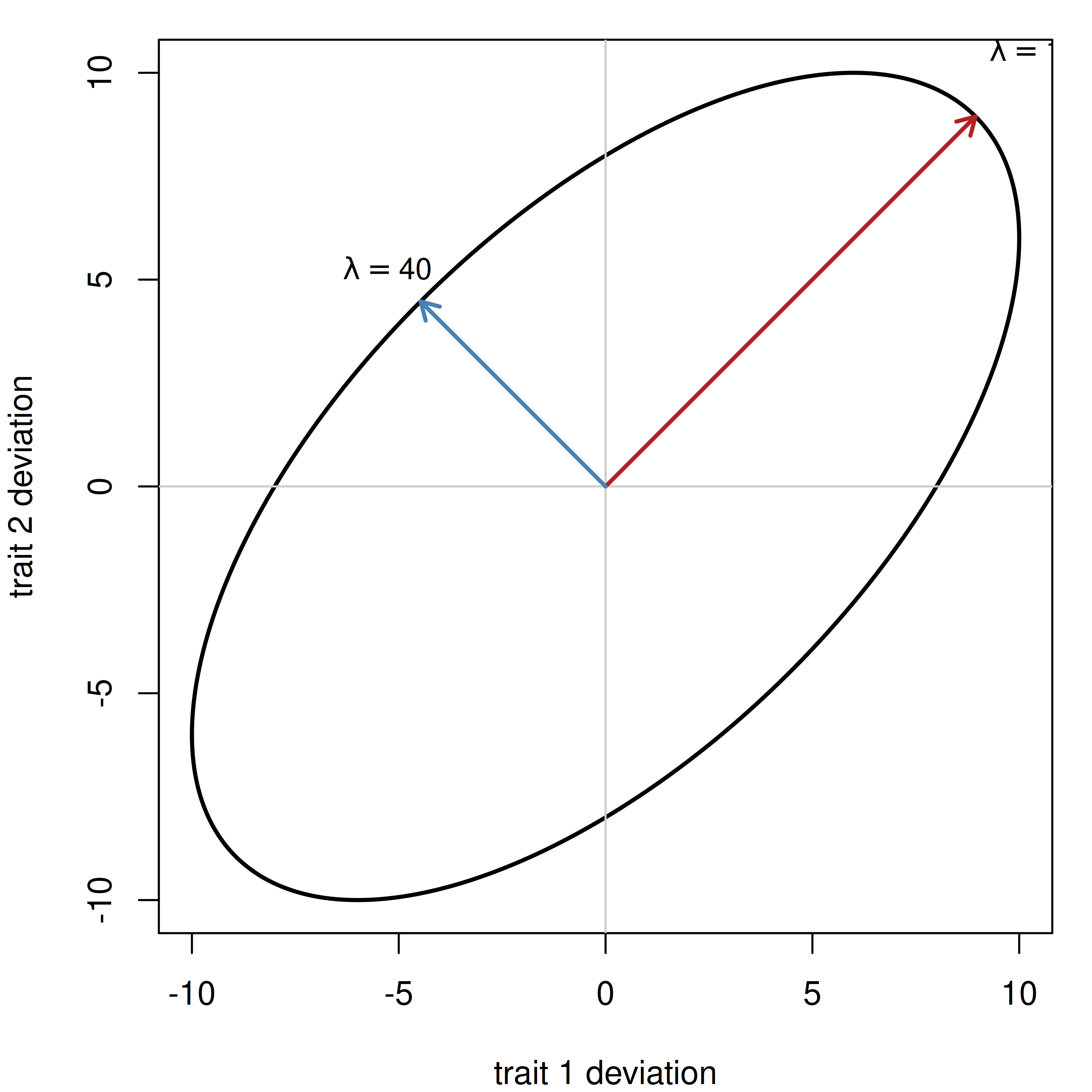
CautionCheck Yourself
The eigenvalues of \mathbf{M} are 160 and 40. Before computing it: what is \det(\mathbf{M}), and what would the determinant be if one eigenvalue were 0?
Answer. 160 \times 40 = 6400, and directly, 100(100) - 60(60) = 10000 - 3600 = 6400. The determinant is the product of the eigenvalues, so a single zero eigenvalue drives the whole determinant to zero — which is §1.8’s singularity seen from a different angle. Likewise the trace (the sum of the diagonal, 100 + 100 = 200) equals the sum of the eigenvalues, 160 + 40 = 200.
Three facts a breeder needs:
- All eigenvalues > 0 means positive definite, which is the condition for a matrix to be a valid covariance matrix. It is the same condition Cholesky tests in §1.12.
NoteDefinition — Positive definite
A symmetric matrix \mathbf{M} is positive definite when every one of its eigenvalues is greater than zero. Equivalently, \mathbf{x}'\mathbf{Mx} > 0 for every non-zero vector \mathbf{x}, and its Cholesky factorisation (§1.12) succeeds. If eigenvalues are zero but none are negative it is positive semi-definite.
Why it matters. A covariance matrix must be positive definite to be a covariance matrix at all. Since \mathbf{x}'\mathbf{Mx} is the variance of a linear combination (§1.15), a non-positive-definite \mathbf{G} would give some index of traits a negative variance, which is impossible. This is what your software means by “G is not positive definite” — a message you will meet in Chapter 21, and one that usually says the data cannot support as many traits as you asked for rather than that the program is broken.
A zero eigenvalue means a perfect genetic correlation. Example C’s singular sibling \begin{bmatrix} 100 & 100 \\ 100 & 100 \end{bmatrix} has eigenvalues 200 and 0: all the variation is on the “together” axis and none on the contrast axis, because r_g = 1 and the two traits are genetically the same trait. REML cannot estimate such a matrix (Chapter 21).
The condition number of §1.8 is the largest eigenvalue over the smallest. For \mathbf{M} that is 160 / 40 = 4. For the near-singular \mathbf{G} of §1.8, with 99.9 in place of 60, the same arithmetic gives 100 + 99.9 = 199.9 and 100 - 99.9 = 0.1, so \kappa = 199.9 / 0.1 = 1999 — the number
kappa()reported. The eigenvalue picture says why: almost all the variation lies along the “together” axis and almost none along the contrast, so the ellipse is a needle, and a needle’s short axis is where rounding error lives.eigen(G)$values # 199.9 and 0.1 #> [1] 199.9 0.1 eigen(G)$values[1] / eigen(G)$values[2] # 1999, the same as kappa(G, exact = TRUE) #> [1] 1999Eigenvectors are the principal components of \mathbf{G}. When a genetic covariance matrix for twenty traits has most of its variance in three eigenvalues, you can model three dimensions instead of twenty. That is what reduced-rank and factor-analytic random regression models do (Chapter 12).
NoteDerivation — why symmetric matrices behave so well (optional)
Skip this on a first read. It explains why every eigenvalue in this book is a real number and every pair of eigenvectors is at right angles — neither of which is true for matrices in general.
Real eigenvalues. Let \mathbf{Mv} = \lambda\mathbf{v} with \mathbf{M} real and symmetric, allowing \lambda and \mathbf{v} to be complex for the moment. Pre-multiply by the conjugate transpose \bar{\mathbf{v}}':
\bar{\mathbf{v}}'\mathbf{M}\mathbf{v} = \lambda\,\bar{\mathbf{v}}'\mathbf{v}
The left side is its own conjugate transpose, because \mathbf{M} is real and symmetric, so it is real. And \bar{\mathbf{v}}'\mathbf{v} = \sum_i |v_i|^2 is real and positive. A real number divided by a positive real number is real, so \lambda is real.
Orthogonal eigenvectors. Take two eigenpairs with \lambda_1 \neq \lambda_2. Then
\lambda_1 \mathbf{v}_2'\mathbf{v}_1 = \mathbf{v}_2'\mathbf{Mv}_1 = (\mathbf{M}\mathbf{v}_2)'\mathbf{v}_1 = \lambda_2 \mathbf{v}_2'\mathbf{v}_1
using \mathbf{M}' = \mathbf{M} in the middle step. So (\lambda_1 - \lambda_2)\mathbf{v}_2'\mathbf{v}_1 = 0, and since the eigenvalues differ, \mathbf{v}_2'\mathbf{v}_1 = 0. The eigenvectors are perpendicular — which is why the ellipse above has axes at right angles, and why the eigen-decomposition \mathbf{M} = \mathbf{V}\boldsymbol{\Lambda}\mathbf{V}' has \mathbf{V}^{-1} = \mathbf{V}'.
Consequences used later. \det(\mathbf{M}) = \prod_j \lambda_j and \operatorname{tr}(\mathbf{M}) = \sum_j \lambda_j both follow from that decomposition, and so does the statement that \mathbf{M} is positive definite exactly when every \lambda_j > 0.
eig <- eigen(M)
eig$values      # 160 and 40
#> [1] 160  40
eig$vectors     # the sum axis and the contrast axis, scaled to length 1
#>           [,1]       [,2]
#> [1,] 0.7071068 -0.7071068
#> [2,] 0.7071068  0.7071068

# The determinant is the product of the eigenvalues.
det(M)
#> [1] 6400
prod(eig$values)
#> [1] 6400

# The trace is their sum.
sum(diag(M))
#> [1] 200
sum(eig$values)
#> [1] 200

# All eigenvalues positive means positive definite: a valid covariance matrix.
all(eig$values > 0)
#> [1] TRUE

# The rg = 1 matrix is not: one eigenvalue is exactly zero.
eigen(matrix(100, nrow = 2, ncol = 2))$values
#> [1] 200   0
A closely related tool, the singular value decomposition, factors any matrix — square or not — as \mathbf{U}\mathbf{D}\mathbf{V}', and for a symmetric positive definite matrix it coincides with the eigen-decomposition. It is the workhorse behind numerically stable rank determination and behind the low-rank approximations used in large-scale evaluation. This book does not develop it; see the companion volume on computation.
1.14 Quadratic forms, traces, and matrix derivatives
This section exists to serve Chapter 21. Variance component estimation by REML is an exercise in differentiating a likelihood with respect to variance components, and the likelihood is built from quadratic forms and traces. Everything here is a tool you will pick up again there. Chapter 2 also needs the last part of it, three pages from now.
1.14.1 Quadratic forms
A quadratic form is \mathbf{x}'\mathbf{Ax} — a row vector, a matrix, and the same vector again as a column. The result is always a single number. The simplest one in this book is the residual sum of squares. From §1.9, the residuals of Example A are
\mathbf{e} = \mathbf{y} - \mathbf{X}\hat{\mathbf{b}} = \begin{bmatrix} 48 \\ 52 \\ 41 \\ 45 \end{bmatrix} - \begin{bmatrix} 50 \\ 50 \\ 43 \\ 43 \end{bmatrix} = \begin{bmatrix} -2 \\ 2 \\ -2 \\ 2 \end{bmatrix}
and
\mathbf{e}'\mathbf{e} = (-2)^2 + 2^2 + (-2)^2 + 2^2 = 16
b_hat <- drop(solve(crossprod(X), crossprod(X, y)))
e <- drop(y - X %*% b_hat)
e
#> [1] -2  2 -2  2

drop(crossprod(e))     # e'e = 16, the residual sum of squares
#> [1] 16
which is \mathbf{e}'\mathbf{Ie}, a quadratic form with \mathbf{A} = \mathbf{I}. Dividing by the residual degrees of freedom, 4 - 2 = 2, gives \hat{\sigma}^2_e = 8 kg².
df <- nrow(X) - qr(X)$rank    # 4 records - 2 estimated effects
df
#> [1] 2
drop(crossprod(e)) / df       # sigma-hat squared = 8
#> [1] 8
The same construction gives \mathbf{y}'\mathbf{y} = 8714 as the uncorrected total sum of squares and \hat{\mathbf{b}}'\mathbf{X}'\mathbf{y} = 43(186) + 7(100) = 8698 as the part explained by the model, and 8714 - 8698 = 16 recovers the residual sum of squares — the sums-of-squares partition Chapter 20 estimates variance components from.
yty      <- drop(crossprod(y))               # total
ss_model <- drop(b_hat %*% crossprod(X, y))  # explained by the model
c(total = yty, model = ss_model, residual = yty - ss_model)
#>    total    model residual
#>     8714     8698       16
1.14.2 Trace
The trace of a square matrix is the sum of its diagonal, \operatorname{tr}(\mathbf{A}) = \sum_i a_{ii}. It equals the sum of the eigenvalues (§1.13), and it has one property that gets used constantly in REML because it permits a reordering that nothing else does:
\operatorname{tr}(\mathbf{AB}) = \operatorname{tr}(\mathbf{BA})
There is no trace() in base R; you sum the diagonal yourself. Check the reordering property on two matrices whose products are plainly different:
AB <- A %*% G0
BA <- G0 %*% A
AB                                                      # not the same matrix
#>      [,1] [,2]
#> [1,]   42 16.5
#> [2,]   30 15.0
BA
#>      [,1] [,2]
#> [1,] 42.0   30
#> [2,] 16.5   15
c(trace_AB = sum(diag(AB)), trace_BA = sum(diag(BA)))   # but the same trace
#> trace_AB trace_BA
#>       57       57
The result worth memorising concerns the hat matrix \mathbf{H} = \mathbf{X}(\mathbf{X}'\mathbf{X})^{-}\mathbf{X}', which turns observations into fitted values: \hat{\mathbf{y}} = \mathbf{Hy}. Its trace equals the rank of \mathbf{X}. For Example A, \operatorname{tr}(\mathbf{H}) = 2, and the residual degrees of freedom are n - \operatorname{tr}(\mathbf{H}) = 4 - 2 = 2 — the same 2 used above. That is where degrees of freedom come from: they count the dimensions the model consumed, and the trace of the projection matrix counts them whether or not \mathbf{X} was full rank.
H <- X %*% solve(crossprod(X)) %*% t(X)

drop(H %*% y)             # the fitted values: 50 50 43 43
#> [1] 50 50 43 43
sum(diag(H))              # trace = 2
#> [1] 2
qr(X)$rank                # the same 2
#> [1] 2
nrow(X) - sum(diag(H))    # residual degrees of freedom
#> [1] 2
1.14.3 Matrix derivatives
Two derivatives, both of a scalar with respect to a vector. The result has the same shape as the vector you differentiated with respect to.
\frac{\partial (\mathbf{a}'\mathbf{x})}{\partial \mathbf{x}} = \mathbf{a} \qquad \frac{\partial (\mathbf{x}'\mathbf{Ax})}{\partial \mathbf{x}} = 2\mathbf{Ax} \quad (\mathbf{A} \text{ symmetric})
The second is the matrix version of \mathrm{d}(ax^2)/\mathrm{d}x = 2ax, which is a good way to remember it. Apply them immediately. Least squares chooses \mathbf{b} to minimise the residual sum of squares, which expands to
(\mathbf{y} - \mathbf{Xb})'(\mathbf{y} - \mathbf{Xb}) = \mathbf{y}'\mathbf{y} - 2\mathbf{b}'\mathbf{X}'\mathbf{y} + \mathbf{b}'\mathbf{X}'\mathbf{Xb}
Differentiate with respect to \mathbf{b}, using the first rule on the middle term and the second on the last (note \mathbf{X}'\mathbf{X} is symmetric), and set the result to zero:
-2\mathbf{X}'\mathbf{y} + 2\mathbf{X}'\mathbf{Xb} = \mathbf{0} \qquad \Longrightarrow \qquad \mathbf{X}'\mathbf{X}\,\hat{\mathbf{b}} = \mathbf{X}'\mathbf{y}
Those are the normal equations, and we have been solving them since §1.9 without having derived them. Chapter 2 opens with the result already in hand.
NoteDerivation — the two matrix derivatives (optional)
Skip this on a first read. Both rules are just ordinary calculus done one element at a time.
Linear form. \mathbf{a}'\mathbf{x} = \sum_k a_k x_k. Differentiating with respect to a single element x_i kills every term except the one containing it:
\frac{\partial}{\partial x_i}\sum_k a_k x_k = a_i
Stacking those partials into a vector gives \mathbf{a}.
Quadratic form. \mathbf{x}'\mathbf{Ax} = \sum_j \sum_k x_j a_{jk} x_k. Element x_i appears in the terms where j = i and in the terms where k = i, so the product rule gives
\frac{\partial}{\partial x_i}\sum_j\sum_k x_j a_{jk} x_k = \sum_k a_{ik}x_k + \sum_j x_j a_{ji}
The first sum is row i of \mathbf{Ax}; the second is row i of \mathbf{A}'\mathbf{x}. In general the derivative is therefore (\mathbf{A} + \mathbf{A}')\mathbf{x}, and when \mathbf{A} is symmetric the two sums are equal and it collapses to 2\mathbf{Ax}. Every quadratic form in this book has a symmetric \mathbf{A} — they are all covariance matrices or crossproducts — so the short version is the one to carry.
1.15 Variances of linear combinations: building V
Almost everything this book computes is a variance of something built out of something else, so this is the most-used result in it.
1.15.1 From one number to many
For a scalar, multiplying a random variable by a constant multiplies its variance by the square of that constant: \mathrm{Var}(ax) = a^2\mathrm{Var}(x). Doubling every breeding value quadruples the genetic variance.
Now the same thing with a matrix. Take three animals — a sire S and his two full-sib progeny, animals 1 and 2 — with additive relationship matrix
\mathbf{A} = \begin{bmatrix} 1 & 0.5 & 0.5 \\ 0.5 & 1 & 0.5 \\ 0.5 & 0.5 & 1 \end{bmatrix} \qquad \mathbf{G} = \mathbf{A}\sigma^2_a = 36\mathbf{A}
Only the two progeny have records, and each has one, so the matrix linking records to animals is
\mathbf{Z} = \begin{bmatrix} 0 & 1 & 0 \\ 0 & 0 & 1 \end{bmatrix}
Two rows, one per record; three columns, one per animal in the pedigree. The sire’s column is all zeros because he has no record of his own.
What is the covariance matrix of the two animals’ breeding values as they appear in the records, \mathrm{Var}(\mathbf{Zu})? Work it out:
\mathbf{ZGZ}' = \begin{bmatrix} 0 & 1 & 0 \\ 0 & 0 & 1 \end{bmatrix} \begin{bmatrix} 36 & 18 & 18 \\ 18 & 36 & 18 \\ 18 & 18 & 36 \end{bmatrix} \begin{bmatrix} 0 & 0 \\ 1 & 0 \\ 0 & 1 \end{bmatrix} = \begin{bmatrix} 36 & 18 \\ 18 & 36 \end{bmatrix}
\mathbf{Z} selected: pre-multiplying picked out the rows of \mathbf{G} belonging to recorded animals, and post-multiplying by \mathbf{Z}' picked out the matching columns. What survives is the sibs’ 2 × 2 corner of \mathbf{G} — the sire’s row and column are gone, and the 18 off the diagonal is 0.5 \times 36, the genetic covariance between full sibs.
What mattered and what did not. The 36 was \sigma^2_a and the 0.5 was the sib relationship — change either and every number changes. The dimensions came from two records and three animals. But the arrangement — pre-multiply by the matrix, post-multiply by its transpose — is what you would do for any \mathbf{Z} at all, and it is the matrix version of squaring the constant.
ImportantKey Equation — Variance of a linear combination
\mathrm{Var}(\mathbf{Ay}) = \mathbf{A}\,\mathrm{Var}(\mathbf{y})\,\mathbf{A}' \tag{1.3}
In words: to get the variance of something built by multiplying, put the multiplier on the left, the original variance in the middle, and the transposed multiplier on the right. The transpose on the right is what keeps the answer square and symmetric.
Here \mathbf{A} is any matrix of constants — this is the one place in the book where that letter is not the relationship matrix. In the worked example above the multiplier was \mathbf{Z}; below it is (\mathbf{X}'\mathbf{X})^{-1}\mathbf{X}'.
1.15.2 Assembling V
Now add the residuals. Each record has residual variance \sigma^2_e = 64, and residuals are independent of each other and of the breeding values, so \mathbf{R} = \mathbf{I}\sigma^2_e and the two variances simply add:
\mathbf{V} = \mathrm{Var}(\mathbf{y}) = \mathbf{ZGZ}' + \mathbf{R} = \begin{bmatrix} 36 & 18 \\ 18 & 36 \end{bmatrix} + \begin{bmatrix} 64 & 0 \\ 0 & 64 \end{bmatrix} = \begin{bmatrix} 100 & 18 \\ 18 & 100 \end{bmatrix}
Every number in \mathbf{V} is something a breeder already knows. The diagonal is the phenotypic variance, 100 kg², so h^2 = 36/100 = 0.36 — Example B’s trait, unchanged. The off-diagonal 18 is the phenotypic covariance between two full sibs, and 18/100 = 0.18 is their phenotypic correlation, which is \tfrac{1}{2}h^2 exactly as sib-analysis theory says it should be.
That is the entire argument of the mixed model, in one matrix. Relationships live in \mathbf{A}; scaling by \sigma^2_a makes them a covariance; \mathbf{Z} propagates them from animals to records; adding \mathbf{R} produces the covariance structure of the data. Chapter 6 does exactly this and then solves.
1.15.3 The variance of an estimate
The same rule gives standard errors. Since \hat{\mathbf{b}} = (\mathbf{X}'\mathbf{X})^{-1}\mathbf{X}'\mathbf{y} is a linear combination of \mathbf{y}, applying Equation 1.3 with \mathrm{Var}(\mathbf{y}) = \mathbf{I}\sigma^2_e and simplifying gives
\mathrm{Var}(\hat{\mathbf{b}}) = (\mathbf{X}'\mathbf{X})^{-1}\sigma^2_e
For a contrast \mathbf{k}'\hat{\mathbf{b}}, one more application gives \mathrm{Var}(\mathbf{k}'\hat{\mathbf{b}}) = \mathbf{k}'(\mathbf{X}'\mathbf{X})^{-1}\mathbf{k}\,\sigma^2_e. For Example A’s flock difference, \mathbf{k} = (0, 1)' picks out the bottom-right element of (\mathbf{X}'\mathbf{X})^{-1}, which is 1, so the variance is 1 \times 8 = 8 and the standard error is \sqrt{8} = 2.83 kg. The 7 kg flock advantage is about 2.5 standard errors from zero — with four lambs, suggestive and no more.
In Chapter 6 the same diagonal, taken from the inverted mixed model coefficient matrix instead, becomes prediction error variance and then accuracy. It is the same calculation throughout.
# A is now the 3 x 3 relationship matrix: sire S, and his two full-sib progeny.
A <- matrix(c(1.0, 0.5, 0.5,
              0.5, 1.0, 0.5,
              0.5, 0.5, 1.0), nrow = 3, byrow = TRUE)

# Z links the two records to their animals. The sire's column is all zeros:
# he has no record of his own.
Z <- matrix(c(0, 1, 0,
              0, 0, 1), nrow = 2, byrow = TRUE)

sigma2_a <- 36
sigma2_e <- 64

G <- A * sigma2_a          # relationships become a covariance matrix
R <- diag(sigma2_e, 2)     # residuals, independent

ZGZt <- Z %*% G %*% t(Z)   # Var(Zu): the sibs' corner of G
ZGZt
#>      [,1] [,2]
#> [1,]   36   18
#> [2,]   18   36

V <- ZGZt + R              # Var(y)
V
#>      [,1] [,2]
#> [1,]  100   18
#> [2,]   18  100

# Everything a breeder reads off V.
sigma2_a / V[1, 1]         # h2 = 0.36
#> [1] 0.36
V[1, 2] / V[1, 1]          # 0.18, the sibs' phenotypic correlation, = h2 / 2
#> [1] 0.18
The simulation is the part a student actually believes. Draw 50,000 sets of breeding values, add residuals, and the realised covariance of the records converges on \mathbf{V}:
set.seed(2024)
n_sim <- 50000

L <- t(chol(G))                                    # section 1.12
u <- L %*% matrix(rnorm(3 * n_sim), nrow = 3)      # breeding values for S, 1, 2
e <- matrix(rnorm(2 * n_sim, sd = sqrt(sigma2_e)), nrow = 2)
y_sim <- Z %*% u + e

round(cov(t(y_sim)), 1)     # converges on V: 100, 18 / 18, 100
#>       [,1] [,2]
#> [1,] 101.3 18.4
#> [2,]  18.4 99.5
And the same rule gives the standard error of the flock contrast from Example A:
k <- c(0, 1)                       # picks out the flock A advantage
XtX_inv <- solve(crossprod(X))
sigma2_e_hat <- 8                  # from section 1.14

var_contrast <- drop(t(k) %*% XtX_inv %*% k) * sigma2_e_hat
var_contrast
#> [1] 8
sqrt(var_contrast)                 # standard error, 2.83 kg
#> [1] 2.828427
1.16 Which section do you need for which chapter?
Nobody reads a matrix algebra chapter straight through and remembers it. Come back here.
| Section | What it gives you | Needed by |
|---|---|---|
| 1.1 Why linear algebra | what it is, and where a breeder meets it | orientation only |
| 1.2 Matrices, vectors, scalars | dimensions, elements, notation, linear combination | all |
| 1.3 Transpose | \mathbf{A}'; symmetry | all |
| 1.4 Addition and scalars | \mathbf{P} = \mathbf{G} + \mathbf{R}; \mathbf{G} = \mathbf{A}\sigma^2_a; \alpha | Ch 3, Ch 6, Ch 11 |
| 1.5 Multiplication | the row-by-column walk; (\mathbf{AB})' = \mathbf{B}'\mathbf{A}' | Ch 2, Ch 6 — the MME itself |
| 1.6 Special matrices | \mathbf{I}, diagonal, symmetric, triangular, block | all |
| 1.7 One model, many animals | \mathbf{y} = \mathbf{Xb} + \mathbf{e}; \mathbf{X}'\mathbf{X} as counts, \mathbf{X}'\mathbf{y} as sums | Ch 2, and every chapter after |
| 1.8 Rank and determinant | why breeding models are singular; the condition number | Ch 2, Ch 5, Ch 21, Ch 24 |
| 1.9 Inversion and partitioning | \mathbf{A}^{-1}; Schur complement; do not invert to solve | Ch 4, Ch 6, Ch 7, Ch 24 |
| 1.10 Generalized inverses | non-unique solutions; estimable functions | Ch 2, Ch 9 |
| 1.11 Kronecker and Hadamard | \mathbf{G}_0 \otimes \mathbf{A}; \mathbf{A} \# \mathbf{A} | Ch 11, Ch 16, Ch 17 |
| 1.12 Cholesky | factorising, simulating, log-determinants | Ch 4, Ch 21, Ch 22, Ch 24 |
| 1.13 Eigenvalues | positive definiteness; principal components | Ch 12, Ch 21 |
| 1.14 Quadratic forms and traces | sums of squares; degrees of freedom; derivatives | Ch 2, Ch 20, Ch 21 |
| 1.15 Variance of a linear combination | \mathbf{V} = \mathbf{ZGZ}' + \mathbf{R}; PEV | Ch 3, Ch 6, Ch 11, Ch 23 |
Sections 1.2 to 1.5 are the ones to read in order. They build on each other — multiplication needs the transpose, and everything after §1.5 needs multiplication. From §1.6 onward you can enter wherever you need to.
If you are heading straight for the animal model in Chapter 6, the minimum is §1.5, §1.9 and §1.15 — but read §1.2 through §1.5 first if you have not done linear algebra before.
1.17 Further reading
Four sources, and when to reach for each.
(Searle 1982), Matrix Algebra Useful for Statistics. If you read one book alongside this chapter, read this one. Searle wrote it for statisticians rather than mathematicians, it covers every operation here in far more depth, and its treatment of rank, generalized inverses and quadratic forms is the natural next step from §1.8, §1.10 and §1.14. Searle took his doctorate in animal breeding under Henderson, which is part of why the examples feel familiar.
(Penrose 1955) and (Rao 1962). The two short papers behind §1.10 — Penrose defines the generalized inverse, Rao shows what it buys you when the normal equations are singular. Read them in that order, and only if you want to know where MASS::ginv() comes from.
(Henderson 1976). The paper that made the animal model practical, by giving rules to write \mathbf{A}^{-1} directly from a pedigree without forming \mathbf{A}. You do not need it yet — Chapter 4 is built on it.
(Wells 2009). An interview rather than a result, and the most readable thing on this list: how matrix algebra, linear models and animal breeding grew up together at Cornell, told by someone who was there.
1.18 Key equations
| Name | Equation | Section |
|---|---|---|
| The reversal rules | Equation 1.1 | §1.5 |
| The inverse of a 2 × 2 | Equation 1.2 | §1.9 |
| Variance of a linear combination | Equation 1.3 | §1.15 |
1.19 Exercises
Solutions are in Appendix H.
Five ewes are weighed. Three are in flock 1, with weights 120, 124 and 131 kg; two are in flock 2, with weights 108 and 112 kg. Using a baseline plus a flock 1 indicator, write \mathbf{X} and \mathbf{y}, then form \mathbf{X}'\mathbf{X} and \mathbf{X}'\mathbf{y} by hand. State in words what every element of each counts or sums. (objective 1)
For two traits, \mathbf{G} = \begin{bmatrix} 16 & 6 \\ 6 & 9 \end{bmatrix} and \mathbf{R} = \begin{bmatrix} 48 & 2 \\ 2 & 16 \end{bmatrix}. Form \mathbf{P}, then compute both heritabilities, the genetic correlation, and the phenotypic correlation. Which of the two traits would respond faster to selection, and why is that not the whole answer? (objective 1)
Take the \mathbf{X}'\mathbf{X} from exercise 1. Compute its determinant, invert it by hand using Equation 1.2, and solve for \hat{\mathbf{b}}. Verify with
solve(), and confirm your two elements against the raw flock means. (objective 1)Six lambs in three flocks of two weigh 50 and 54; 44 and 48; 39 and 41 kg. Build the overparameterised \mathbf{X} with a baseline and all three flock columns. Show it is rank deficient and give its rank. Then produce two different generalized-inverse solutions, show that the fitted values agree, and give one estimable function on which they agree. (objective 2)
With \mathbf{G}_0 = \begin{bmatrix} 36 & 12 \\ 12 & 9 \end{bmatrix} for two traits and \mathbf{A} the relationship matrix of three animals — a sire and two of his half-sib progeny out of unrelated dams — form both \mathbf{G}_0 \otimes \mathbf{A} and \mathbf{A} \otimes \mathbf{G}_0. In each, identify the element that is \mathrm{cov}(a_{1,\,\text{trait }1},\, a_{3,\,\text{trait }2}), and say which ordering each matrix uses. (objective 3)
Let \mathbf{G} = \begin{bmatrix} 64 & 24 \\ 24 & 25 \end{bmatrix} be a genetic covariance matrix for two traits.
- Compute its Cholesky factor \mathbf{L} by hand, entry by entry, and verify \mathbf{LL}' = \mathbf{G}. (objective 4)
- In R, use \mathbf{L} to simulate 10,000 pairs of correlated breeding values and confirm that the realised covariance matrix recovers \mathbf{G}. Remember that
chol()returns the upper factor. (objective 4) - Those 10,000 animals are each measured once for trait 1, so \mathbf{Z} = \mathbf{I} and \mathbf{R} = \mathbf{I}\sigma^2_e with \sigma^2_e = 36. Use Equation 1.3 to give \mathrm{Var}(\mathbf{Zu}) and then \mathbf{V} for trait 1, and state the heritability. (objective 5)