| Category | Species | Trait | Typical Value | Heritability (h²) |
|---|---|---|---|---|
| Production | Swine | ADG (25-110 kg) | 850-950 g/d | 0.30-0.40 |
| Dairy | 305-d milk yield | 10,000 kg | 0.30-0.40 | |
| Beef | Weaning weight | 220 kg | 0.30-0.40 | |
| Broilers | Body weight (42d) | 2.6 kg | 0.30-0.50 | |
| Layers | Eggs/hen (18-80 wk) | 330 eggs | 0.25-0.35 | |
| Reproduction | Swine | NBA (born alive) | 12-14 pigs | 0.10-0.15 |
| Dairy | Daughter pregnancy rate | 20% | 0.03-0.05 | |
| Beef | Heifer pregnancy | 90% | 0.10-0.15 | |
| Layers | Age at first egg | 19 wk | 0.40-0.50 | |
| Health/Fitness | Dairy | Somatic cell score | 3.0-3.5 | 0.10-0.15 |
| Swine | PRRS resistance | Variable | 0.15-0.30 | |
| Broilers | Leg soundness score | 1.5 (0-5 scale) | 0.05-0.20 | |
| Efficiency | Swine | RFI (feed efficiency) | -0.05 kg/d | 0.30-0.45 |
| Beef | RFI (feedlot) | -0.2 kg/d | 0.30-0.45 | |
| Layers | Feed per dozen eggs | 1.6 kg | 0.25-0.40 | |
| Quality | Swine | Backfat depth | 12 mm | 0.40-0.60 |
| Beef | Marbling score | 5.5 (3-8 scale) | 0.35-0.50 | |
| Layers | Egg weight | 62 g | 0.50-0.60 |
2 Selection Basics
Learning Objectives
By the end of this chapter, you will be able to:
- Define phenotype and distinguish it from genotype
- Explain the importance of accurate phenotyping in animal breeding
- Describe challenges in recording and managing livestock data
- Articulate how breeding objectives guide selection decisions
- Understand the concept of True Breeding Value (TBV)
2.1 Introduction
In Chapter 1, you learned about the structure of the animal breeding industry—the breeding pyramids, the companies, the revenue streams, and the technologies that enable genetic improvement. Now we turn to the practical foundation of every breeding program: What are we actually trying to improve, and how do we measure it?
Imagine you’re a geneticist at a swine breeding company. Your team has been tasked with improving growth rate in your terminal sire line. This sounds straightforward—select faster-growing pigs as parents. But as you’ll discover in this chapter, this seemingly simple goal raises many critical questions:
- What trait exactly should we measure? Body weight at a specific age? Average daily gain over a period? Weight at a target backfat depth?
- How do we measure it accurately? Manual weighing? Automated scales? How often?
- How do we record and manage the data? What if an ID tag is misread or a weight is entered incorrectly?
- Is growth rate the only thing that matters? What about feed efficiency, carcass quality, leg soundness, or meat quality?
- How do we know which pigs are genetically superior vs. just raised in a better environment?
This chapter addresses these foundational questions. We’ll explore:
- Traits of economic importance: The characteristics that drive profitability in livestock production
- Phenotypes and phenotyping: What we observe and how we measure it accurately
- Data recording and management: The critical infrastructure that makes breeding programs work
- Breeding objectives: Defining what traits to improve and their relative importance
- True Breeding Value (TBV): The concept of genetic merit that underpins all selection decisions
By the end of this chapter, you’ll understand that successful animal breeding depends not just on sophisticated statistical models (which we’ll cover in later chapters), but on high-quality data collected systematically over time. As the saying goes: “Garbage in, garbage out.” Without accurate phenotypes and clear breeding objectives, no amount of statistical wizardry can produce genetic progress.
Let’s begin by exploring the traits that matter in livestock breeding.
2.2 Traits of Economic Importance
Not all traits are created equal when it comes to livestock breeding. Some traits directly determine revenue (milk sold, eggs produced, carcass weight), while others affect costs (feed consumption, veterinary treatments, mortality). Still others influence long-term sustainability (longevity, welfare, environmental impact).
Traits of economic importance can be organized into six major categories. As we explore each category, notice how the same principles apply across species, but the specific traits and their relative importance vary by production system.
2.2.1 2.1 Production Traits
Production traits are the most visible and often the most emphasized—they directly determine the quantity of product (meat, milk, eggs) an animal produces.
Growth Rate
Growth rate measures how quickly an animal gains body weight over time. It’s critical for meat-producing species where animals are raised to a target market weight.
Common measurements:
Average Daily Gain (ADG): Body weight gain per day over a defined period \[\text{ADG} = \frac{\text{Final Weight} - \text{Initial Weight}}{\text{Days on Test}}\]
Body weight at fixed age: E.g., broiler weight at 42 days, pig weight at 150 days
Species-specific examples:
| Species | Trait | Typical Range | Units |
|---|---|---|---|
| Swine | ADG from 25-110 kg | 800-1,000 g/day | g/day |
| Broilers | Body weight at 42 days | 2.4-2.8 kg | kg |
| Beef cattle | Weaning weight (adjusted 205d) | 180-250 kg | kg |
| Beef cattle | Yearling weight (adjusted 365d) | 350-450 kg | kg |
| Layers | Body weight at 18 weeks | 1.3-1.5 kg | kg |
Economic importance: Faster growth means: - Shorter time to market (reduced facility and labor costs) - More production cycles per year - Greater throughput and revenue
However, there can be trade-offs: Extremely fast growth can lead to leg problems (broilers), increased backfat (swine), or metabolic issues.
Milk Yield
For dairy cattle, milk production is the primary revenue-generating trait.
Measurement: - 305-day lactation yield: Total milk produced in first 305 days of lactation (kg) - Test-day records: Monthly milk weights via DHI (Dairy Herd Improvement) testing or daily via automated milking systems
Typical values: - Elite Holsteins: 10,000-14,000 kg per 305-day lactation - Average Holsteins (USA): ~10,000 kg - Jersey cattle: 6,000-8,000 kg (but higher components)
Economic importance: At $0.35-0.45 per kg milk, a cow producing 1,000 kg more per lactation generates $350-450 extra revenue.
However, genetic selection for extremely high milk yield has been associated with: - Reduced fertility (longer days open, lower conception rates) - Increased metabolic disorders (ketosis, displaced abomasum) - Shorter productive life (more culling)
This is why modern breeding objectives balance milk yield with health and fertility (more on this in Section 2.5).
Egg Production
For laying hens, the number of eggs produced over the hen’s productive life determines revenue.
Measurement: - Eggs per hen housed: Total eggs from point of housing (e.g., 18 weeks) to end of lay cycle (e.g., 80 weeks) - Peak production: Maximum eggs per 100 hens per day (e.g., 95-98%) - Persistency: Maintenance of production after peak
Typical values: - Modern commercial layers: 320-350 eggs per hen housed (18-80 weeks) - Peak rates: 95-98 eggs per 100 hens per day
Economic importance: At $0.10-0.15 per egg (farm gate), an extra 20 eggs per hen = $2.00-3.00 additional revenue per hen.
Egg production is highly heritable (h² ≈ 0.25-0.35), making it responsive to selection. However, breeders must also consider: - Egg weight: Larger eggs have premium value but may reduce total egg numbers - Shell quality: Cracked eggs are unsellable - Feed efficiency: Feed costs dominate layer economics
Feed Intake
While not a traditional “production” trait, feed intake is measured extensively because it’s necessary for calculating feed efficiency (Section 2.4).
Measurement: - Daily feed intake (kg/day or g/day) - Cumulative feed intake over test period
Technologies: - Electronic feeders: FIRE systems (swine), GrowSafe (cattle), automated poultry feeders - RFID-enabled: Each animal identified when accessing feeder, intake recorded automatically
Typical values: - Growing-finishing pigs (25-110 kg): 1.8-2.5 kg/day - Dairy cows (lactating): 20-28 kg dry matter/day - Broilers (1-42 days): Cumulative ~3.5-4.5 kg - Beef steers (feedlot): 10-14 kg dry matter/day
2.2.2 2.2 Reproductive Traits
Reproductive traits determine how many offspring an animal produces over its lifetime. These traits are economically critical but present unique breeding challenges—they typically have low heritability (h² < 0.15) and are often sex-limited (expressed only in one sex).
Litter Size (Swine)
Litter size measures the number of offspring born per litter in polytocous species (those that produce multiple offspring).
Common measurements: - Total born (TB): Total piglets born (alive + stillborn) - Number born alive (NBA): Live piglets at birth - Number weaned (NW): Piglets surviving to weaning (~21 days)
Typical values (modern commercial sows): - Total born: 13-16 piglets - Born alive: 12-14 piglets - Weaned: 11-13 piglets
Economic importance: At $50 per weaned pig, one extra pig weaned per litter × 2.3 litters per sow per year = $115 extra revenue per sow per year.
Breeding challenge: Litter size has very low heritability (h² ≈ 0.10-0.15), meaning: - Most variation is environmental (sow condition, nutrition, management) - Genetic progress is slow - Requires large datasets and accurate pedigrees - Genomic selection helps increase accuracy
Fertility
Fertility encompasses the ability to conceive and maintain pregnancy.
Common measurements:
| Species | Trait | Definition | Typical Value |
|---|---|---|---|
| Dairy | Daughter Pregnancy Rate (DPR) | % pregnant per 21-day cycle | 18-25% |
| Dairy | Days Open | Days from calving to conception | 100-150 days |
| Beef | Heifer Pregnancy (HP) | % heifers pregnant at ~14 months | 85-95% |
| Beef | First Service Conception Rate | % pregnant after first insemination | 50-65% |
| Swine | Farrowing rate | % of mated sows that farrow | 85-90% |
| Layers | Sexual maturity | Age at first egg | 18-20 weeks |
Economic importance: - Dairy: Each extra day open costs ~$3-5 (delayed lactation, increased breeding costs) - Beef: Open cows generate no calf crop and still incur maintenance costs
Heritability: Generally low (h² ≈ 0.03-0.10 for most fertility traits), making improvement difficult but not impossible with genomic selection and large datasets.
Calving/Farrowing Ease
Dystocia (difficult birth) causes calf/piglet mortality, maternal injury, and increased labor.
Measurement: - Calving ease score: 1 (unassisted) to 5 (extreme difficulty, caesarean section) - Birth weight: Often used as predictor (heavier calves/piglets → more dystocia) - Percentage unassisted births
Typical values: - Beef cattle: 85-95% unassisted births (heifers lower) - Dairy: 90-95% unassisted births - Swine: Farrowing duration, stillborn rate (indicator)
Heritability: - Direct calving ease (calf’s effect): h² ≈ 0.05-0.15 - Maternal calving ease (cow’s pelvic capacity): h² ≈ 0.10-0.20
Breeding strategy: Select terminal sires with negative EPD for birth weight (smaller, easier-born calves), especially for use on heifers.
2.2.3 2.3 Health and Fitness Traits
Health traits are increasingly important in breeding programs as producers, consumers, and regulators focus on animal welfare and reducing antibiotic use.
Disease Resistance
Disease resistance measures an animal’s ability to avoid infection or minimize disease severity.
Examples by species:
| Species | Disease | Measurement | Heritability |
|---|---|---|---|
| Dairy | Mastitis | Somatic Cell Score (SCC) | h² ≈ 0.10-0.15 |
| Dairy | Lameness | Mobility score, foot lesions | h² ≈ 0.05-0.15 |
| Swine | PRRS resistance | Viremia, weight loss | h² ≈ 0.15-0.30 |
| Poultry | Newcastle disease | Antibody titer, mortality | h² ≈ 0.10-0.30 |
| Salmon | IPN (infectious pancreatic necrosis) | Survival post-challenge | h² ≈ 0.15-0.40 |
Measurement challenges: - Disease challenge tests: Expensive, require controlled exposure - Natural disease incidence: Depends on pathogen exposure (environmental) - Genomic selection: Increasingly used for disease traits (identify resistant genotypes without challenge)
Economic importance: - Mastitis (dairy): ~$200-300 per case (treatment, milk loss, culling) - PRRS (swine): ~$5-10 per pig in mortality, reduced growth - Diseases reduce animal welfare and necessitate antibiotic use
Longevity and Stayability
Longevity measures how long an animal remains productive in the herd.
Common measurements: - Productive life (dairy): Months from first calving to culling - Stayability (beef): Probability cow remains in herd to age 6, having weaned 5+ calves - Survival (poultry): Mortality rate from housing to end of lay
Typical values: - Dairy: Average productive life ~2.5-3.5 lactations (goal: >4) - Beef: Stayability to age 6: ~60-75% - Layers: Mortality 18-80 weeks: 3-8%
Economic importance: - Dairy: Each extra lactation = ~$500-1,000 saved (replacement cost, calf value) - Beef: Cows that stay in herd longer amortize their development costs over more calves
Heritability: Low to moderate (h² ≈ 0.05-0.15), but selection indices increasingly include longevity due to its economic impact.
2.2.4 2.4 Efficiency Traits
Efficiency traits measure how effectively animals convert inputs (primarily feed) into outputs (meat, milk, eggs). With feed representing 60-70% of production costs, efficiency is economically critical.
Feed Efficiency: RFI vs. FCR
There are two main ways to express feed efficiency:
1. Feed Conversion Ratio (FCR)
\[\text{FCR} = \frac{\text{Feed Intake}}{\text{Body Weight Gain}}\]
- Lower FCR is better (less feed per kg gain)
- Typical values:
- Broilers: 1.5-1.8 kg feed per kg gain
- Swine: 2.4-2.8 kg feed per kg gain
- Beef cattle: 5.5-7.5 kg feed per kg gain
Limitation: FCR is confounded with growth rate. Fast-growing animals naturally have better FCR (less feed for maintenance per kg gain).
2. Residual Feed Intake (RFI)
RFI is the difference between an animal’s actual feed intake and its expected feed intake based on body weight and gain.
\[\text{RFI} = \text{Actual Feed Intake} - \text{Expected Feed Intake}\]
- Negative RFI is better (eats less than expected for its size and growth)
- RFI is independent of growth rate (you can select for low RFI without reducing growth)
Example (swine): - Pig A: Grows 900 g/day, eats 2.0 kg/day → Expected intake: 2.1 kg/day → RFI = 2.0 - 2.1 = -0.1 kg/day (efficient!) - Pig B: Grows 900 g/day, eats 2.4 kg/day → Expected intake: 2.1 kg/day → RFI = 2.4 - 2.1 = +0.3 kg/day (inefficient)
Heritability: - FCR: h² ≈ 0.25-0.40 - RFI: h² ≈ 0.30-0.45
Why measure RFI? RFI is more expensive to measure (requires individual feed intake), but it allows: - Selection for efficiency without reducing growth - Improved profitability: Reducing RFI by 0.1 kg/day = ~5-8 kg less feed per pig (~$2-3 saved)
Partial Efficiency Traits
- Feed per kg milk (dairy): kg dry matter intake per kg milk produced
- Feed per dozen eggs (layers): kg feed per 12 eggs
- Residual energy intake (dairy): Similar to RFI, accounting for milk production and body weight change
2.2.5 2.5 Quality Traits
Quality traits determine product value—consumers and processors pay premiums for higher-quality products.
Carcass Composition (Meat Animals)
Key traits:
| Trait | Species | Measurement | Typical Range |
|---|---|---|---|
| Backfat depth | Swine | Ultrasound, carcass | 10-18 mm |
| Loin depth | Swine | Ultrasound, carcass | 50-70 mm |
| Marbling score | Beef | Visual, camera grading | 3-8 (USDA scale) |
| Ribeye area | Beef | Carcass measurement | 75-95 cm² |
| Breast meat yield | Broilers | Processing plant data | 21-26% of live weight |
| Percent lean | Swine | Calculated from carcass | 55-62% |
Economic importance: - Swine: Each mm less backfat = ~$0.50-1.00 per carcass (leaner = higher value) - Beef: Marbling score increase (Choice to Prime) = $50-150 premium per carcass - Broilers: 1% increase in breast yield = ~$0.05-0.10 per bird
Heritability: Moderate to high (h² ≈ 0.30-0.60), making carcass traits highly responsive to selection.
Milk Components (Dairy)
Milk is priced based on component content, not just volume.
Key traits: - Fat %: Typically 3.5-4.5% in Holsteins, 4.5-6.0% in Jerseys - Protein %: Typically 3.0-3.5% in Holsteins, 3.5-4.0% in Jerseys - Fat yield (kg): Total kg fat = % × milk yield - Protein yield (kg): Total kg protein = % × milk yield
Economic importance: Milk payment formulas often reward components more than volume. Example: - $0.30 per kg milk + $2.50 per kg fat + $4.00 per kg protein
Genetic correlations: - Milk yield vs. fat%: Negative (r_A ≈ -0.3 to -0.5) — selecting for volume reduces % - Milk yield vs. fat kg: Positive (r_A ≈ +0.5 to +0.7) — more volume = more total fat - Fat% vs. protein%: Positive (r_A ≈ +0.6) — tend to move together
Egg Quality (Layers)
Key traits: - Egg weight: 55-65 g (premium for larger eggs, but size must fit carton) - Shell strength: Breaking force (kg), shell thickness (mm) - Shell color: Brown vs. white (market preference, no quality difference) - Internal quality: Albumin height, Haugh units (measure of freshness) - Yolk color: Fan score (1-15), driven by diet and genetics
Economic importance: - Cracked eggs: 6-10% loss; shell strength reduces cracks - Egg size: Premium for large/extra-large grades
Heritability: Generally moderate to high (h² ≈ 0.30-0.60 for most egg quality traits).
Meat Quality
-
pH: Ultimate pH (pHu) after rigor mortis — affects water-holding capacity, color
- Swine: Normal pHu = 5.6-5.8; PSE (pale, soft, exudative) if < 5.4
- Color: L* (lightness), a* (redness), b* (yellowness) — consumer preference for darker red meat
- Tenderness: Warner-Bratzler shear force (lower = more tender) — major quality factor in beef
- Intramuscular fat: Marbling — associated with tenderness, flavor, juiciness
Heritability: Moderate (h² ≈ 0.20-0.50 for most meat quality traits).
2.2.6 2.6 Welfare Traits
Animal welfare is increasingly important to consumers, retailers, and regulations. Welfare traits are challenging to define and measure but are entering breeding programs.
Temperament and Behavior
Measurement: - Temperament scores: Docility during handling (1 = calm, 5 = aggressive) - Flight speed: Time to exit a chute (cattle) — faster = more excitable - Fear response: Tonic immobility test (poultry), open field test
Typical heritability: h² ≈ 0.10-0.40 depending on trait and measurement method
Economic importance: - Cattle: Calm temperament improves safety for handlers, reduces stress-induced weight loss - Swine: Aggressive pigs cause injuries, tail biting - Poultry: Feather pecking and cannibalism reduce welfare and productivity
Leg and Foot Health
Leg problems are a major welfare concern, especially in fast-growing broilers and high-producing dairy cows.
Examples: - Broilers: Leg scores (gait analysis, 0 = normal to 5 = severe lameness) - Dairy: Locomotion scores (1 = sound to 5 = severely lame) - Swine: Leg soundness, osteochondrosis
Heritability: Low to moderate (h² ≈ 0.05-0.20)
Selection challenge: Leg problems are often genetically correlated with production traits: - Broilers: Fast growth → heavier body weight → increased leg stress - Dairy: High milk yield → increased metabolic stress → increased lameness risk
Modern breeding programs use multi-trait selection to balance production with leg health.
Absence of Genetic Defects
Some welfare issues are caused by deleterious recessive alleles. Examples: - Cattle: Hypotrichosis (hairlessness), chondrodysplasia (dwarfism) - Dogs: Hip dysplasia, progressive retinal atrophy, brachycephalic syndrome
Breeding strategy: - DNA testing: Identify carriers of recessive alleles - Mating strategies: Avoid carrier × carrier matings (produces affected offspring) - Selection against carriers: Gradually reduce allele frequency
2.2.7 2.7 Summary Table: Key Traits by Species
The table below summarizes economically important traits across major livestock species, providing typical values and approximate heritabilities. These values will become more meaningful as we cover heritability in detail in Chapter 5.
Why Heritability Matters
Heritability (h²) is the proportion of phenotypic variation due to additive genetic effects (Chapter 5). Key takeaways:
- High heritability (h² > 0.40): Traits respond quickly to selection (growth, carcass, egg weight)
- Moderate heritability (h² = 0.20-0.40): Steady progress possible (milk yield, feed efficiency)
- Low heritability (h² < 0.20): Slow progress, requires large datasets and genomic tools (fertility, disease resistance)
Notice that reproductive and health traits typically have low heritability—this is why modern breeding increasingly relies on genomic selection to improve accuracy for these difficult traits.
2.3 Phenotypes and Phenotyping
Now that we’ve identified what traits matter, we turn to the practical challenge of measuring them accurately. This process—called phenotyping—is the foundation of all genetic improvement. Without high-quality phenotypes, genetic evaluations will be biased, selection decisions will be wrong, and genetic progress will stall.
As you’ll see in this section, phenotyping is far more than simply “weighing a pig” or “counting eggs.” It requires careful attention to measurement protocols, equipment calibration, data recording, and quality control.
2.3.1 3.1 What is a Phenotype?
A phenotype is any observable or measurable characteristic of an organism. In animal breeding, phenotypes are the traits we record on individual animals—body weight, milk yield, egg production, backfat depth, disease incidence, temperament, and so on.
Definition:
Phenotype: The observable expression of an animal’s genotype in a specific environment.
Mathematically, we can express the phenotype as:
\[P = G + E\]
Where: - P = Phenotype (what we observe and measure) - G = Genotype (genetic contribution, sum of all genetic effects) - E = Environment (all non-genetic factors: nutrition, management, health, weather, measurement error)
We’ll formalize this model in Chapter 3 by partitioning the genetic component (\(G\)) into additive, dominance, and epistatic effects. For now, the key insight is that phenotype ≠ genotype. An animal with a high phenotype may be:
- Genetically superior (large \(G\))
- In a favorable environment (large positive \(E\))
- Both
- Lucky (random environmental advantage)
Example: Two pigs, both weighing 110 kg at 150 days of age
-
Pig A: Comes from a genetically superior line (parents had high EBVs), raised in average conditions
- \(G\) = high, \(E\) = average → \(P\) = 110 kg
-
Pig B: Comes from average parents (moderate EBVs), raised in exceptionally favorable conditions (best pen, extra feeding attention)
- \(G\) = average, \(E\) = high → \(P\) = 110 kg
Both pigs have identical phenotypes (110 kg), but Pig A is the better breeding animal because its phenotype reflects superior genetics, not just favorable environment. The challenge of animal breeding is to estimate \(G\) from \(P\), which requires accounting for environmental variation.
2.3.2 3.2 Measurement Accuracy and Precision
Not all phenotypic measurements are created equal. The quality of phenotypic data depends on two distinct properties: accuracy and precision.
Accuracy
Accuracy measures how close a measurement is to the true value.
- High accuracy: Measurements are close to the true value on average
- Low accuracy: Measurements are systematically biased (e.g., scale consistently reads 2 kg too high)
Sources of inaccuracy: - Uncalibrated equipment (scales, ultrasound machines) - Systematic measurement errors (always weighing pigs in the afternoon when gut fill is higher) - Observer bias (subjective scoring)
Precision
Precision measures the repeatability of measurements—how close repeated measurements are to each other.
- High precision: Repeated measurements give similar results
- Low precision: Repeated measurements vary widely
Sources of imprecision: - Measurement error (animal movement during weighing, variable ultrasound probe placement) - Temporal variation (weighing at different times of day) - Observer variation (different technicians scoring the same animal differently)
The Target Analogy
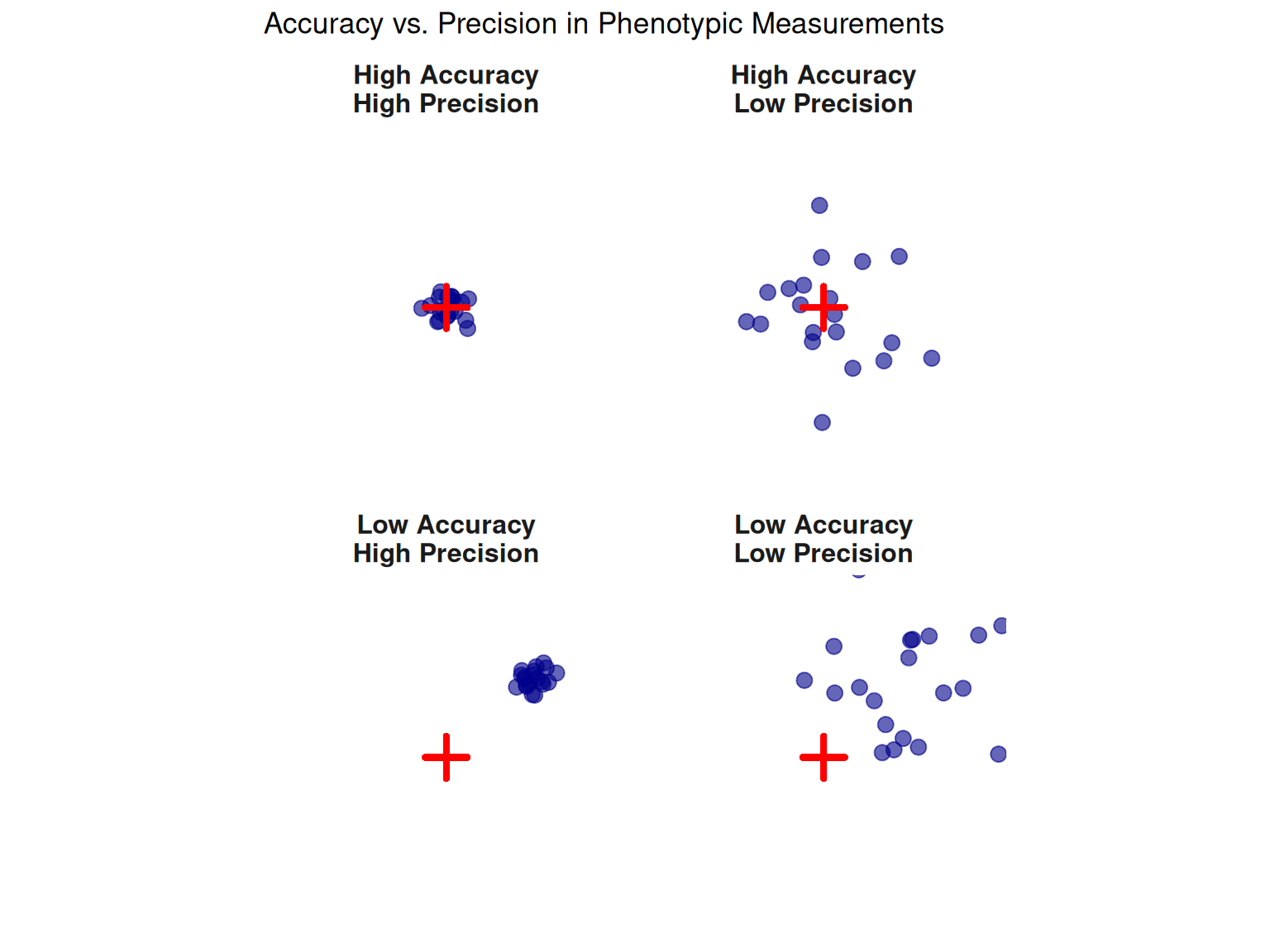
Why it matters in breeding:
Accuracy: Biased measurements lead to biased EBVs and incorrect selection decisions. For example, if a scale always reads 5 kg too high, pigs weighed on that scale appear genetically superior when they’re not.
Precision: Imprecise measurements inflate the environmental variance (\(\sigma^2_E\)), which reduces the effective heritability and slows genetic progress.
Goal: Breeding programs strive for high accuracy and high precision—measurements that are both correct on average and repeatable.
2.3.3 3.3 Challenges in Phenotyping Livestock
Accurate phenotyping is often the most expensive and time-consuming aspect of a breeding program. Let’s explore the main challenges.
Cost
Modern phenotyping technologies can be prohibitively expensive:
| Technology | Purpose | Approximate Cost |
|---|---|---|
| Electronic feeder (FIRE system, swine) | Individual feed intake | $50,000-$100,000+ per pen (10-12 pigs) |
| GrowSafe feeder (cattle) | Individual feed intake | $60,000-$120,000 per pen |
| Automated milking system (dairy) | Milk yield, components, health | $150,000-$250,000 per robot |
| Ultrasound machine (carcass) | Backfat, loin depth | $15,000-$40,000 |
| CT/MRI scanner | High-resolution carcass composition | $500,000-$2,000,000+ |
| Genomic SNP chip | Genotyping for genomic selection | $30-$150 per animal |
Trade-off: Companies must balance the cost of phenotyping against the genetic gain achieved by having more accurate data. For example:
- Installing electronic feeders to measure feed efficiency costs ~$5,000-8,000 per pig phenotyped
- But selecting for RFI can save $2-4 per market pig in feed costs
- With millions of market pigs produced annually, the investment pays off over time
Time
Some traits require months or years to measure:
- Longevity (dairy): Requires cows to complete multiple lactations (4-8 years)
- Stayability (beef): Requires cows to reach age 6 and wean multiple calves
- Feed efficiency (RFI): Requires 8-12 weeks of daily intake records per animal
- Carcass traits: Require slaughter (can’t select the best animals—they’re dead!)
Solution: Use correlated traits measured earlier or on relatives: - Ultrasound carcass traits on live animals (correlated with actual carcass) - Genomic selection (predict EBVs using DNA markers, no need to wait for phenotypes) - Progeny testing (measure trait on relatives, not the selection candidate)
Invasiveness
Some phenotypes require invasive or destructive procedures:
- Carcass traits: Require slaughter
- Internal organs: Require necropsy (research context, disease resistance studies)
- Blood samples: Immune assays, metabolic profiles
- Biopsies: Muscle samples for meat quality analysis
Invasive phenotypes are often measured on a subset of animals (progeny, siblings), and their information is used to predict breeding values for the live selection candidates via genetic relationships.
Throughput
Manual phenotyping is labor-intensive and limits the number of animals that can be measured:
- Manual milk recording (dairy): Technician records each cow’s milk yield (slow, only monthly)
- Trap nests (layers): Manually identify which hen laid which egg (labor-intensive)
- Carcass dissection: Extremely time-consuming, limited to research settings
Solution: Automation dramatically increases throughput: - Milking robots: Record every cow, every milking (2-3× per day) - RFID nest boxes: Automatically detect which hen enters each nest - Camera-based phenotyping: Automated body condition scoring, weight estimation (Chapter 25)
2.3.4 3.4 Examples by Species
Let’s explore how major livestock species phenotype their most important traits, highlighting the technologies and challenges involved.
Swine Breeding
Growth traits (body weight, ADG): - Measurement: Electronic scales at entry to finishing barn and at market - Frequency: Initial weight (~25 kg), final weight (~110-130 kg) - Challenge: Pigs housed in groups, so individual weighing requires sorting - Automation: Walk-through scales, automated sorting gates
Feed efficiency (RFI): - Measurement: FIRE (Feed Intake Recording Equipment) feeders - How it works: RFID ear tag identifies pig, feeder records feed disappearance each visit - Duration: 8-12 weeks of data collection per pig - Challenge: Expensive ($50K-100K per pen), requires careful management - Benefit: Individual feed intake enables direct selection for RFI (saves $2-3 per pig in feed costs)
Backfat and loin depth (carcass quality): - Measurement: Real-time ultrasound at ~100 kg body weight - Location: Between 10th-11th rib (standard site) - Technician training: Requires skilled ultrasound operator - Accuracy: Correlation with carcass measurements: r ≈ 0.70-0.85
Litter size (reproduction): - Measurement: Manual counting at farrowing (birth) - Timing: Within 24-48 hours of birth - Traits recorded: Total born, born alive, stillborn, mummified - Challenge: Requires accurate sow and piglet identification, 24/7 farrowing supervision
Dairy Cattle Breeding
Milk yield: - Traditional (DHI testing): Monthly milk weights recorded by technician - Technician visits farm once per month - Weighs milk from each cow at one milking - Adjusted to 305-day lactation yield using standardized curves - Modern (automated milking systems - AMS): Milking robot records every milking - Each cow milked 2-3× per day voluntarily - Continuous data stream: yield, milking time, flow rate - More accurate estimates, enables selection for milking speed
Milk components (fat%, protein%): - DHI testing: Lab analysis from monthly test-day samples - AMS: Inline sensors (near-infrared spectroscopy) measure components in real-time - Accuracy: Inline sensors slightly less accurate than lab but provide daily data
Fertility: - Traits: Days open (calving to conception), daughter pregnancy rate, first-service conception - Measurement: Breeding records, pregnancy checks (palpation, ultrasound) - Challenge: Requires accurate record-keeping of inseminations and calving dates
Health (mastitis, lameness): - Somatic cell count (SCC): Indicator of mastitis (elevated SCC = infection) - Measured from monthly DHI test-day samples - Also measured at bulk tank level (herd average) - Lameness: Locomotion scoring (1-5 scale), mobility assessments - Subjective, requires trained observer - Computer vision systems (Chapter 25) increasingly used for automated lameness detection
Poultry Breeding (Broilers)
Body weight: - Measurement: Group weighing (sample of birds from pen) or individual weighing - Age: Typically at 35-42 days (market age) - Challenge: Handling stress can affect weight; standardized protocols required
Feed efficiency (FCR): - Measurement: Group level (pen) - Total feed consumed by pen ÷ total weight gain of pen - Limitation: Can’t measure individual bird feed intake in typical commercial housing - Genomic selection: Increasingly used to predict individual FCR using DNA markers
Carcass traits (breast yield, leg yield, abdominal fat): - Measurement: Processing plant data (post-slaughter) - Selection challenge: Must select on family information (can’t measure on the selection candidate itself) - Modern: CT scans on live birds (research settings), genomic prediction
Leg health: - Measurement: Gait scoring (0 = normal to 5 = severe lameness) - Challenge: Subjective, requires standardized scoring protocols - Economic importance: Lame birds have reduced welfare, lower growth, higher mortality
Poultry Breeding (Layers)
Egg production: - Traditional: Trap nests—hen enters nest, door closes, eggs collected and identified to hen - Labor-intensive, stressful for hens - Modern: RFID nest boxes—hen’s leg band automatically identified when entering nest - Automated recording, less stressful - Eggs per hen housed, persistency of lay
Egg quality: - Egg weight: Automated inline scales as eggs move on conveyor - Shell strength: Deformation test, breaking force - Sample of eggs per hen, measured in lab - Shell color: Visual or automated color grading - Internal quality: Haugh units (albumin height relative to egg weight) - Sample of eggs broken and measured
Feed efficiency: - Measurement: Feed per dozen eggs or feed per kg of egg mass - Challenge: Measuring individual feed intake is difficult in cage-free systems - Genomic selection: Enables selection for feed efficiency without expensive individual measurements
Beef Cattle Breeding
Growth traits (weaning weight, yearling weight): - Measurement: Scales at weaning (~205 days) and yearling (~365 days) - Adjustments: Standardized to 205-day and 365-day weights using age-adjustment factors - Contemporary groups: Animals compared within herd-year-season groups
Carcass traits: - Live animal ultrasound: Backfat, ribeye area, intramuscular fat (marbling) - Measured at ~365 days (yearling age) or pre-slaughter - Correlation with actual carcass: r ≈ 0.60-0.80 - Actual carcass data: From progeny or siblings sent to slaughter - Marbling score, yield grade, carcass weight, ribeye area - Most accurate but requires slaughter (can’t select the animal itself)
Feed efficiency (RFI): - Measurement: GrowSafe feeders (individual feed intake in feedlot) - Challenge: Extremely expensive, limited to seedstock herds and research - Duration: 70-120 days of feed intake data per animal - Adoption: Low (~1-2% of beef industry), primarily genomic prediction used instead
Maternal traits: - Measurement: Weaning weight of calves (maternal ability), calving ease scores, cow size - Challenge: Traits expressed only in females, requires multiple breeding seasons - EPDs: Maternal milk EPD, maternal calving ease EPD
2.4 Recording and Managing Data
Phenotyping produces vast amounts of data—millions of records across thousands or millions of animals. This data is the lifeblood of a breeding program. Without systematic data recording, quality control, and management, even the best phenotyping technologies are useless.
This section covers the practical systems that enable breeding programs to collect, validate, store, and retrieve phenotypic data reliably.
2.4.1 4.1 Animal Identification Systems
Before we can record a phenotype, we must know which animal it belongs to. Animal identification is therefore the first essential step in data management.
Visual Identification
Ear tags: - Plastic or metal tags attached to the ear with unique numbers - Pros: Inexpensive ($0.50-$2 per tag), easy to apply, visible from distance - Cons: Can be lost, difficult to read when dirty, prone to fading, not suitable for automated data capture
Tattoos: - Permanent ink applied inside ear or on skin - Pros: Permanent, cannot be removed or lost - Cons: Hard to read without restraint, fades over time, requires good technique
Branding: - Hot iron or freeze branding on hide - Pros: Permanent, visible from distance - Cons: Painful, damages hide (reduces carcass value), welfare concerns, increasingly discouraged
Species-specific considerations: - Cattle: Visual ear tags most common, some brands still used in range cattle - Swine: Ear notching (historical, rare now), ear tags - Sheep: Ear tags, paint marks (temporary) - Poultry: Leg bands (layers), wing bands, no ID (broilers, group selection)
Electronic Identification (RFID)
Radio Frequency Identification (RFID) uses a microchip that transmits a unique ID when scanned by a reader.
Passive RFID: - No battery: Powered by electromagnetic field from reader - Range: Short (typically <1 meter) - Applications: Ear tags (cattle, swine), leg bands (poultry), injectable transponders - Cost: $2-$5 per tag
Active RFID: - Battery powered: Transmits continuously or on schedule - Range: Longer (up to 100+ meters) - Applications: Location tracking, estrus detection collars (dairy) - Cost: $15-50+ per tag
How RFID works in breeding programs:
- Animal approaches automated system (feeder, scale, milking robot, nest box)
- RFID reader detects tag and reads unique ID
- System records phenotype (feed intake, body weight, milk yield, egg) linked to that animal’s ID
- Data automatically uploaded to database
Example: Swine feed efficiency (RFI) - Each pig wears an RFID ear tag with unique ID - FIRE feeder reads tag when pig enters - Feed disappearance recorded for that specific pig - 8-12 weeks of data → calculate individual RFI - No manual recording required!
Benefits: - Automation: Eliminates manual data entry (reduces errors) - High throughput: Thousands of records per day - Real-time data: Immediate upload to database - Accuracy: No transcription errors
Challenges: - Tag loss: 1-5% of tags lost (animals lose ears in fights, tags fall out) - Misreads: Electronic interference, dirty tags - Cost: Higher initial investment than visual ID
DNA-Based Parentage Verification
Even with careful record-keeping, pedigree errors occur: - Incorrect sire recorded (wrong bull/boar used) - Dam mis-identified (piglet assigned to wrong sow) - Sample swaps in lab (genotype or phenotype mislabeled)
Pedigree errors bias breeding value estimates and reduce genetic gain.
DNA parentage testing: - Microsatellite markers (historical) or SNP panels (modern) - Compare offspring genotype to putative parents - If genotypes incompatible → pedigree error detected
When used: - Routine verification: Genotype all selection candidates and verify parentage (common in swine, poultry breeding companies) - Natural mating: Assign paternity when multiple sires per pen (beef, sheep) - Quality control: Detect sample swaps or recording errors
Cost-benefit: - Cost: ~$20-$50 per animal (using SNP chips that also provide genomic data) - Benefit: Correcting even 2-5% pedigree errors significantly improves EBV accuracy and genetic gain
2.4.2 4.2 Data Entry and Validation
Even with automated systems, human data entry is often required—especially for reproductive traits, health events, and management records.
Common Data Entry Errors
| Error Type | Example | Impact |
|---|---|---|
| Transposed digits | Animal 1234 recorded as 1243 | Phenotype assigned to wrong animal |
| Wrong date | Birth date entered as 2024-02-30 (impossible) | Invalid record, breaks age calculations |
| Unit errors | Weight in pounds entered as kg (or vice versa) | Severely biased phenotype |
| Decimal errors | 1.5 kg entered as 15 kg | Extreme outlier |
| Swapped IDs | Phenotypes for animals A and B accidentally swapped | Both animals get wrong phenotypes |
| Missing data | Required field left blank | Record unusable for analysis |
| Duplicate records | Same phenotype entered twice | Inflates sample size, biases estimates |
Validation Rules
Range checks: - Birth weight must be within biologically plausible range (e.g., 0.5-2.5 kg for piglets) - Egg weight must be 40-80 g (anything outside → flag for review) - Milk yield per day < 80 kg (higher values likely errors)
Date sequence checks: - Birth date < Weaning date < Current date - Insemination date < Calving date (and gestation ~280 days for cattle)
ID verification: - Animal ID must exist in database before phenotype can be entered - Parent IDs must exist if recording pedigree - No duplicate IDs
Logical consistency: - Can’t have litter size of 0 (sow either farrowed or didn’t) - Can’t have male with lactation record
Implementation: - Database constraints: Enforce rules at database level (prevent invalid entries) - Entry forms: Use dropdown menus, date pickers, range validators - Real-time feedback: Alert user immediately if entry violates rule
Timeliness
Enter data as soon as possible after collection: - Same day is best (memory fresh, fewer errors) - Delays lead to: Lost paper records, forgotten values, transcription errors
Digital data capture: - Tablet or phone apps at point of measurement (enter directly into device) - Automated systems upload in real-time - Eliminates paper → digital transcription step (major source of errors)
###4.3 Data Quality Control
Even with validation rules, errors slip through. Quality control (QC) is the systematic process of identifying and correcting errors in existing data.
Outlier Detection
Statistical outliers are observations that are far from the population mean—they may be: 1. Real biological extremes (keep in dataset) 2. Measurement errors (investigate and correct or remove)
Common method: ±3 SD rule
- Calculate mean (\(\bar{y}\)) and standard deviation (\(s\)) for a trait within contemporary group
- Flag values outside \(\bar{y} \pm 3s\)
- Review flagged records: Are they plausible? Or errors?
Example (swine weaning weight): - Contemporary group: 100 piglets weaned at 21 days - Mean weight: \(\bar{y} = 6.2\) kg - Standard deviation: \(s = 0.8\) kg - Flagging rule: Flag any piglet < 3.8 kg or > 8.6 kg
Suppose one piglet shows 12.0 kg → Likely error (probably 1.2 kg entered as 12.0 kg). Investigate!
Impossible Values
Some errors are obvious: - Negative body weights - Birth date after measurement date - Litter size > 25 piglets (biologically implausible) - Milk yield > 100 kg/day (Holstein average is ~30-40 kg/day)
Automated checks can flag these for review.
Duplicate Records
Sometimes the same phenotype is entered twice (e.g., technician forgot they already entered it): - Check for identical animal ID + trait + date + value - Remove duplicates (keep only one copy)
Missing Data Patterns
Random missing data: A few animals missing records due to chance → usually not a problem
Systematic missing data: Can bias genetic evaluations - Example: Only sick animals get health records → makes disease look more common than it is - Example: Smallest piglets not weighed (too small to handle) → inflates average weaning weight
Solution: Ensure complete data collection for all animals in contemporary groups whenever possible.
2.4.3 4.4 Database Structures (Brief Introduction)
Modern breeding programs store data in relational databases—systems that organize data into tables linked by keys.
Core Tables
1. Animals Table
| Column | Description | Example |
|---|---|---|
| animal_id | Unique identifier | PIG_12345 |
| sire_id | Father’s ID | BOAR_789 |
| dam_id | Mother’s ID | SOW_456 |
| birth_date | Date of birth | 2024-03-15 |
| sex | M or F | F |
| breed | Breed code | DUROC |
2. Phenotypes Table
| Column | Description | Example |
|---|---|---|
| animal_id | Links to Animals table | PIG_12345 |
| trait_code | Which trait | BW_WEAN |
| value | Measured value | 6.5 |
| unit | Unit of measurement | kg |
| date | Measurement date | 2024-04-05 |
| contemporary_group | Environmental grouping | FARM1_2024_SPRING_PEN3 |
3. Genotypes Table
| Column | Description | Example |
|---|---|---|
| animal_id | Links to Animals table | PIG_12345 |
| snp_chip | Chip version | PorcineSNP60v2 |
| marker_1 | Genotype at marker 1 | 0 (AA) |
| marker_2 | Genotype at marker 2 | 1 (AB) |
| … | … | … |
| marker_50000 | Genotype at marker 50000 | 2 (BB) |
Why relational databases? - No redundancy: Each piece of information stored once, linked by IDs - Data integrity: Enforce relationships (e.g., phenotype can’t exist for non-existent animal) - Efficient queries: Extract data for genetic evaluation using SQL (Structured Query Language)
Example SQL query (extract weaning weights for pigs born in 2024):
SELECT a.animal_id, a.birth_date, p.value AS weaning_weight
FROM animals a
JOIN phenotypes p ON a.animal_id = p.animal_id
WHERE p.trait_code = 'BW_WEAN'
  AND a.birth_date >= '2024-01-01'
  AND a.birth_date < '2025-01-01';
We’ll cover databases and SQL in more detail in Chapter 14 (Practical Skills). For now, the key takeaway: Structured data storage is essential for managing breeding program data at scale.
2.5 Breeding Objectives
We’ve covered what traits exist (Section 2) and how to measure them (Sections 3-4). Now we address a critical strategic question: What should we actually select for?
This question defines the breeding objective (also called the breeding goal)—the traits we want to improve and their relative importance. Defining a clear breeding objective is essential because:
- Resources are limited: We can’t measure everything on every animal
- Trade-offs exist: Some traits are genetically antagonistic (improving one worsens another)
- Priorities differ: Different production systems have different economic drivers
2.5.1 5.1 Defining the Breeding Goal
The breeding goal should reflect the economic reality of the production system. Ask:
- What traits drive revenue? (milk sold, pigs weaned, eggs produced, carcass weight)
- What traits drive costs? (feed consumption, veterinary treatments, mortality, days to market)
- What are the constraints? (regulations, animal welfare standards, market demands, sustainability goals)
Formal definition:
The breeding goal (H) is a linear combination of traits weighted by their economic importance:
\[H = v_1 \cdot \text{BV}_1 + v_2 \cdot \text{BV}_2 + \cdots + v_n \cdot \text{BV}_n\]
Where: - \(H\) = Aggregate breeding value (overall genetic merit) - \(v_i\) = Economic weight for trait \(i\) ($/unit improvement) - \(\text{BV}_i\) = Breeding value for trait \(i\)
We’ll formalize this in Chapter 9 (Selection Index). For now, understand that economic weights determine how much we value improvement in each trait.
Example (simplified dairy breeding goal):
\[H = 0.30 \cdot \text{Milk} + 2.50 \cdot \text{Fat kg} + 4.00 \cdot \text{Protein kg} - 3.00 \cdot \text{Days Open} + 8.00 \cdot \text{Productive Life}\]
This says: - Each extra kg of milk is worth $0.30 - Each extra kg of fat is worth $2.50 - Each extra kg of protein is worth $4.00 - Each day reduction in days open is worth $3.00 - Each extra month of productive life is worth $8.00
2.5.2 5.2 Single Trait vs. Multiple Trait Selection
Single Trait Selection
Single trait selection focuses on improving one trait, ignoring all others.
When it’s appropriate: - Research context: Studying response to selection for a specific trait - Extreme scenarios: One trait dominates economic value (rare in commercial breeding)
Example: Selecting only for egg production in layers - Benefit: Fast progress in egg numbers - Problem: Correlated traits may deteriorate: - Egg weight may decrease (negative genetic correlation) - Shell quality may decline - Feed efficiency may worsen - Mortality may increase (metabolic stress)
Result: Short-term gain in eggs, long-term problems with profitability and welfare.
Multiple Trait Selection
Multiple trait selection simultaneously improves several traits, accounting for economic importance and genetic correlations.
Why it’s necessary: - Profitability depends on multiple traits, not just one - Genetic correlations mean selecting for one trait affects others - Balance is essential: Can’t maximize production at the expense of reproduction, health, or welfare
Approach: - Selection index: Combine traits into single value (H) that predicts economic merit - Optimal weights: Account for economic values, heritabilities, and genetic correlations - Selection decision: Rank animals by index value, select the top percentage
We’ll develop selection index theory in Chapter 9.
2.5.3 5.3 Economic Weights (Introduction)
Economic weights quantify the value of a one-unit genetic improvement in a trait, holding all other traits constant.
Formal definition:
\[v_i = \frac{\partial \text{Profit}}{\partial \text{BV}_i}\]
This is the partial derivative of profit with respect to the breeding value for trait \(i\).
In plain language: If we could magically increase an animal’s breeding value for trait \(i\) by 1 unit (1 kg, 1 day, 1 egg, etc.), how much would lifetime profit change?
Example (swine): - Economic weight for ADG: +$15 per 100 g/day improvement - Faster growth → fewer days to market → lower facility/labor costs → more turns per year - Economic weight for feed efficiency (RFI): -$30 per 0.1 kg/day improvement in RFI - Lower RFI (more efficient) → less feed consumed → major cost savings (feed = 60-70% of costs) - Economic weight for backfat: -$8 per 1 mm reduction - Leaner carcasses receive premium pricing
Deriving economic weights: Economic weights are derived from profit equations that model the production system:
\[\text{Profit} = \text{Revenue} - \text{Costs}\]
For swine: \[\text{Profit} = (\text{Carcass Weight} \times \text{Price per kg}) - (\text{Feed Cost} + \text{Fixed Costs})\]
By taking partial derivatives with respect to each trait’s breeding value, we get economic weights.
We’ll work through detailed examples in Chapter 9. For now, recognize that economic weights: - Differ by production system (dairy, beef, terminal swine vs. maternal swine) - Change over time (as market prices, costs, and regulations change) - Require careful analysis (not just guesswork!)
2.5.4 5.4 Examples of Breeding Objectives by Species
Let’s explore real-world breeding objectives for major livestock species. Notice how objectives differ by production role (maternal vs. terminal, milk vs. beef, etc.).
Dairy Cattle: Net Merit Index (NM$)
Purpose: Maximize lifetime profit of a cow’s daughters
Traits included (simplified; actual index has 20+ traits):
| Trait | Economic Weight | Why It Matters |
|---|---|---|
| Milk yield (kg) | +$0.02-0.04 per kg | Revenue from milk sales |
| Fat yield (kg) | +$2.00-3.00 per kg | Component pricing (fat valued highly) |
| Protein yield (kg) | +$3.50-5.00 per kg | Component pricing (protein most valuable) |
| Productive life (months) | +$8-12 per month | Reduce replacement costs, more lactations |
| Daughter pregnancy rate (%) | +$15-25 per % | Reduce days open, more calves, lower breeding costs |
| Somatic cell score | -$50-80 per unit increase | Mastitis indicator; higher SCC = milk loss, treatments |
| Body size composite | -$1-3 per unit | Larger cows eat more feed (maintenance cost) |
Key insights: - Components valued more than volume: Protein yield has ~100× higher weight than milk yield per unit - Fertility matters: Despite low heritability, fertility has high economic weight - Health is economically important: Mastitis resistance (low SCC) is highly valued - Size has negative weight: Bigger ≠ better (higher maintenance costs)
Historical shift: - Pre-2000: Selection focused almost exclusively on milk yield - Result: Milk production increased dramatically, but fertility, health, and longevity declined - Post-2000: Balanced selection via Net Merit → stabilized fertility and health while continuing milk yield progress
Swine: Maternal vs. Terminal Lines
Swine breeding programs maintain separate lines with different breeding objectives:
Maternal Line Objective (Large White, Landrace):
Goal: Maximize sow productivity and longevity
| Trait | Emphasis | Why |
|---|---|---|
| Number born alive (NBA) | High | More piglets = more revenue |
| Piglet survival to weaning | High | No value if piglets die |
| Maternal ability (milk production) | High | Heavier weaning weights |
| Longevity | High | Sows cost $200-300 to develop; need 4-6 parities to pay off |
| Feed efficiency | Moderate | Important but less than reproduction |
| Growth rate | Low | Maternal gilts not slaughtered (growth less critical) |
| Carcass leanness | Low | Not slaughtered for meat |
Terminal Sire Line Objective (Duroc, Pietrain):
Goal: Maximize efficiency and carcass value of market offspring
| Trait | Emphasis | Why |
|---|---|---|
| Growth rate (ADG) | High | Faster to market = lower costs, more throughput |
| Feed efficiency (RFI) | Very High | Feed costs dominate; RFI improvement = major savings |
| Carcass leanness (low backfat) | High | Lean carcasses receive premium |
| Loin depth / muscle | High | More saleable meat per carcass |
| Meat quality (pH, color) | Moderate | Affects consumer acceptance |
| Litter size | None | Terminal sires mated to F₁ females (sire’s litter size doesn’t matter for commercial production) |
Why separate lines? - Trade-offs: Selection for extreme growth and leanness can reduce reproductive fitness - Crossbreeding: Maternal line gilts crossed with terminal sires → commercial pigs get both maternal advantages (from dam) and growth/carcass advantages (from sire)
Broiler Chickens
Goal: Fast, efficient growth to market weight with good carcass yield and acceptable leg health
| Trait | Emphasis | Economic Weight Context |
|---|---|---|
| Body weight at 42 days | Very High | More meat sold per bird |
| Feed conversion ratio (FCR) | Very High | Feed = 60-70% of costs |
| Breast meat yield (%) | High | Breast is most valuable cut |
| Leg health / soundness | Moderate | Welfare concern; lame birds grow slower |
| Livability (survival) | High | Dead birds = total loss |
| Uniformity | Moderate | Easier processing if birds similar size |
Challenge: Genetic correlation between growth and leg problems - Fast growth → heavier body weight → more stress on immature leg bones → higher lameness - Solution: Multi-trait selection index that balances growth with leg health
Industry progress: - 1950s: Broilers required 16-18 weeks to reach 2 kg, FCR ≈ 4.0 - 2020s: Broilers reach 2.6-2.8 kg in 6 weeks, FCR ≈ 1.6-1.8 - Genetic gain: ~60-80 g per year increase in body weight, ~0.02-0.03 improvement in FCR per year
Laying Hens
Goal: Maximize egg production with good egg quality and feed efficiency
| Trait | Emphasis | Why |
|---|---|---|
| Eggs per hen housed | Very High | Primary revenue source |
| Egg weight | High | Premium for larger eggs (but not too large for cartons) |
| Shell strength | High | 6-10% breakage rate; stronger shells = fewer cracks |
| Feed efficiency | High | Feed cost per dozen eggs critical for profit |
| Persistency of lay | Moderate | Maintain production after peak |
| Livability | High | Mortality reduces eggs per hen housed |
| Feather cover / pecking | Moderate | Welfare and production issue |
Trade-off: Egg production vs. egg weight - Genetic correlation: r_A ≈ -0.2 to -0.4 (antagonistic) - Selecting for more eggs tends to reduce average egg weight - Solution: Include both in index with appropriate weights
Beef Cattle: Terminal vs. Maternal
Like swine, beef cattle breeding distinguishes terminal and maternal objectives.
Terminal Sire Index (for bulls mated to produce slaughter calves):
| Trait (EPD) | Emphasis | Why |
|---|---|---|
| Yearling weight | High | Heavier calves at sale |
| Carcass weight | High | More meat = more revenue |
| Marbling score | High | Premium for Choice/Prime grades |
| Ribeye area | High | More high-value cuts |
| Calving ease (direct) | Moderate | Avoid dystocia when bull used on heifers |
| Birth weight | Negative | Lower birth weight = easier calving |
Maternal Index (for replacement heifers and cows):
| Trait (EPD) | Emphasis | Why |
|---|---|---|
| Heifer pregnancy rate | High | Must breed to be productive |
| Calving ease (maternal) | High | Cow must calve unassisted |
| Milk (maternal milk EPD) | Moderate | Better milk = heavier weaning weights in calves |
| Stayability | High | Cows that last 6+ years amortize development costs |
| Mature cow size | Negative | Smaller cows = lower feed costs (maintenance) |
| Docility | Moderate | Calm cows safer to handle |
2.6 True Breeding Value (TBV)
We’ve now covered traits, phenotyping, data management, and breeding objectives. But there’s one critical concept we haven’t yet defined: What exactly is it that we’re trying to select for?
The answer is the True Breeding Value (TBV)—the genetic merit of an animal as a parent. Understanding TBV is fundamental to everything that follows in this course.
2.6.1 6.1 Definition of True Breeding Value
True Breeding Value (TBV) is defined as:
The sum of the average effects of all alleles an individual carries, summed across all loci that affect a trait.
More precisely:
\[\text{TBV} = \sum_{i=1}^{n} \alpha_i\]
Where: - \(n\) = number of loci affecting the trait - \(\alpha_i\) = average effect of the allele at locus \(i\) that the individual carries
In simpler terms: TBV represents twice the expected deviation of an animal’s offspring from the population mean, assuming the animal is mated to average individuals.
Why “twice”? Because an offspring receives half its genes from each parent. So if a parent’s TBV is +10 kg, its offspring will be +5 kg above average (on average), assuming the other parent is average.
TBV vs. Phenotype: A Critical Distinction
- Phenotype (P): What we observe and measure on the animal itself
- TBV: The genetic value the animal passes to its offspring
These are not the same! An animal with a high phenotype may have: - High TBV (genetically superior) - Favorable environment (good pen, extra feed, optimal health) - Both
Only TBV is heritable—passed to offspring.
Example: Two dairy cows, both producing 12,000 kg milk per lactation
- Cow A: TBV = +500 kg, Environment = +500 kg → Phenotype = 12,000 kg
- Cow B: TBV = +1,000 kg, Environment = 0 kg → Phenotype = 12,000 kg
Both cows produce the same milk, but Cow B is the superior breeding animal. Her daughters will average +500 kg more milk than Cow A’s daughters (each inherits half the dam’s TBV, plus half from the sire).
2.6.2 6.2 Why TBV is Important
TBV is the target of selection because:
- TBV is heritable: An animal passes (on average) half its TBV to each offspring
- TBV predicts offspring performance: Animals with high TBV produce superior offspring
- TBV breeds true: Unlike environmental effects, TBV is permanent and transmitted across generations
- TBV determines genetic progress: Selecting high-TBV parents creates cumulative genetic gain
Contrast with environmental effects:
- Favorable environment (best pen, extra nutrition, optimal health) improves an animal’s phenotype but doesn’t pass to offspring
- High TBV improves the animal’s phenotype and passes half to each offspring, creating permanent improvement
This is why we spend so much effort estimating TBV (Chapter 7) and designing selection programs to maximize genetic gain (Chapter 6).
2.6.3 6.3 TBV is Unknown but Estimable
Here’s the challenge: We can never observe TBV directly.
TBV is a theoretical construct—the sum of effects of alleles we can’t see (unless we sequence the genome and know the effect of every variant, which we don’t). We only observe phenotypes, which are a mixture of genetics and environment:
\[P = \text{TBV} + E\]
(We’ll formalize this more carefully in Chapter 3, partitioning genetics into additive, dominance, and epistatic components.)
So how do we estimate TBV?
We use information that is correlated with TBV:
-
Animal’s own phenotype: Imperfect (includes environmental effects), but informative
- Correlation with TBV depends on heritability: \(r = \sqrt{h^2}\)
-
Pedigree information: Parents, grandparents, siblings
- Parents pass half their TBV to offspring
- Full sibs share 50% of genes, half-sibs share 25%
-
Progeny performance: Offspring inherit half their parent’s TBV
- Highly informative, especially if many progeny measured
-
Genomic information: DNA markers (SNPs) linked to causal genes
- Captures Mendelian sampling variation (Chapter 13)
- Enables prediction at birth, before phenotypes available
By combining all this information using statistical models (BLUP, genomic BLUP), we produce Estimated Breeding Values (EBVs):
\[\text{EBV} \approx \text{TBV}\]
EBVs are our best guess at an animal’s true genetic merit. The accuracy of the EBV depends on how much information we have:
- Low accuracy (r ≈ 0.30-0.50): Young animal, no progeny, no genomic data
- Moderate accuracy (r ≈ 0.50-0.70): Own phenotype, pedigree, or genomic data
- High accuracy (r ≈ 0.80-0.95): Many progeny tested, or genomic data + extensive phenotyping
We’ll cover EBV estimation in detail in Chapter 7.
2.6.4 6.4 Ranking Animals by TBV
The goal of selection is simple:
Rank animals by their TBV and select the top-ranked individuals as parents.
In practice, since we don’t know TBV, we:
- Estimate TBV using available information → produces EBVs
- Rank animals by EBV (or by a selection index combining multiple EBVs)
- Select the top percentage (e.g., top 10%, top 1%) as parents
- Mate selected parents to produce the next generation
- Repeat the process, accumulating genetic gain over generations
Example: Selecting replacement gilts in swine
A breeding company evaluates 1,000 candidate gilts. For each gilt, they have: - Phenotypes: Growth rate, backfat, litter size of dam - Pedigree: Known parents, grandparents - Genomic data: Genotyped with 60K SNP chip
They run a genetic evaluation (BLUP + genomic prediction) to estimate EBVs for each trait, then compute a selection index combining traits with economic weights.
Result: Each gilt gets a single index value (estimate of aggregate TBV, \(H\)).
Selection: Top 100 gilts (10%) selected as replacement breeding stock.
Outcome: The selected gilts have higher average TBV than the unselected gilts → next generation has higher genetic merit → genetic progress.
2.6.5 6.5 Conceptual Diagram: Phenotype, TBV, and Environment
Let’s visualize the relationship between phenotype, TBV, and environment for a hypothetical trait (e.g., body weight at 150 days in swine).
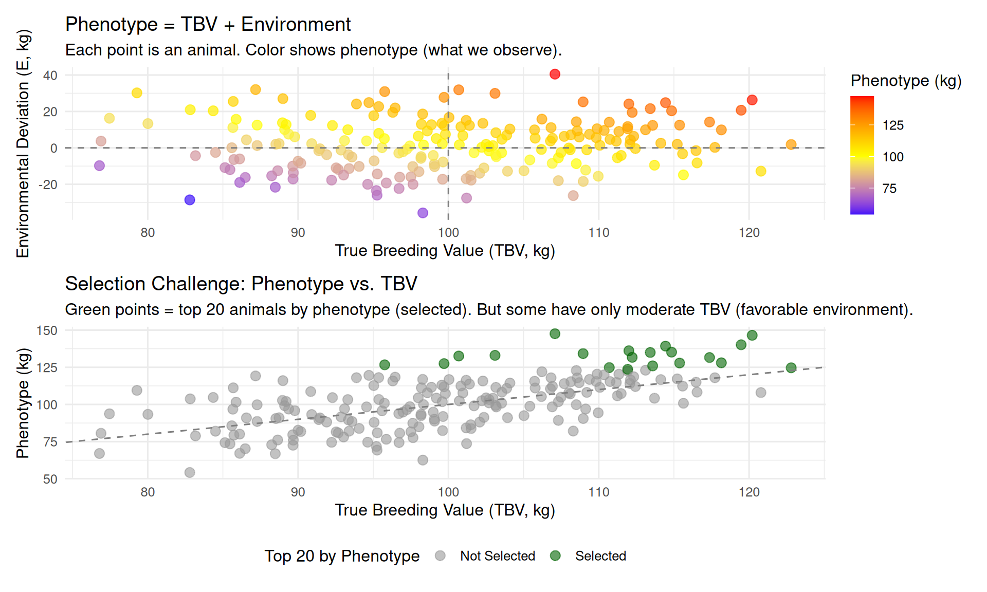
Key insights from the diagram:
- Phenotype is the sum of TBV and environment: Animals with identical phenotypes can have very different TBVs
- Selection on phenotype alone is imperfect: Some animals with high phenotypes have only moderate TBV (they benefited from favorable environments)
- Goal of genetic evaluation: Use all available information (own performance, relatives, genomic data) to separate TBV from environmental effects and rank animals accurately
The Central Challenge of Animal Breeding
We want to select animals with high TBV, but we can only observe phenotypes (which include environmental effects).
The entire machinery of quantitative genetics—heritability, genetic correlations, BLUP, genomic selection—exists to solve this problem: How do we accurately estimate TBV from noisy phenotypic data?
2.7 R Code Demonstrations
Let’s reinforce the concepts from this chapter with some practical R examples. These demonstrations will show you how to load, visualize, and quality-check phenotypic data.
2.7.1 Demo 1: Loading and Summarizing Phenotypic Data
# Load packages
library(tidyverse)

# Simulate a dataset of swine growth data
# (In a real breeding program, you'd load this from a database)
set.seed(789)

n_pigs <- 500

swine_data <- tibble(
  pig_id = paste0("PIG_", 1001:(1000 + n_pigs)),
  sire_id = sample(paste0("BOAR_", 1:20), n_pigs, replace = TRUE),
  dam_id = paste0("SOW_", sample(1:100, n_pigs, replace = TRUE)),
  birth_date = as.Date("2024-01-15") + sample(0:60, n_pigs, replace = TRUE),
  sex = sample(c("M", "F"), n_pigs, replace = TRUE),
  pen = sample(paste0("PEN_", 1:10), n_pigs, replace = TRUE),
  birth_weight = rnorm(n_pigs, mean = 1.4, sd = 0.3),
  weaning_weight = rnorm(n_pigs, mean = 6.5, sd = 1.2),
  final_weight = rnorm(n_pigs, mean = 110, sd = 12),
  backfat = rnorm(n_pigs, mean = 13, sd = 2.5)
)

# Summary statistics
cat("Summary of Swine Growth Data:\n")
Summary of Swine Growth Data:Number of pigs: 500 cat("Number of sires:", n_distinct(swine_data$sire_id), "\n")Number of sires: 20 cat("Number of dams:", n_distinct(swine_data$dam_id), "\n")Number of dams: 100 cat("Number of pens:", n_distinct(swine_data$pen), "\n\n")Number of pens: 10 # Summarize key traits
summary_stats <- swine_data %>%
select(birth_weight, weaning_weight, final_weight, backfat) %>%
summary()
print(summary_stats) birth_weight weaning_weight final_weight backfat
Min. :0.5507 Min. : 1.721 Min. : 78.62 Min. : 3.978
1st Qu.:1.2008 1st Qu.: 5.702 1st Qu.:103.16 1st Qu.:11.279
Median :1.3798 Median : 6.541 Median :110.83 Median :12.991
Mean :1.3892 Mean : 6.461 Mean :111.14 Mean :12.982
3rd Qu.:1.5732 3rd Qu.: 7.228 3rd Qu.:120.20 3rd Qu.:14.776
Max. :2.2892 Max. :10.136 Max. :148.42 Max. :19.694 2.7.2 Demo 2: Data Visualization
# Distribution of final weight
p1 <- ggplot(swine_data, aes(x = final_weight)) +
  geom_histogram(bins = 30, fill = "steelblue", color = "black", alpha = 0.7) +
  geom_vline(xintercept = mean(swine_data$final_weight),
             linetype = "dashed", color = "red", size = 1) +
  labs(title = "Distribution of Final Weight",
       subtitle = paste("Mean =", round(mean(swine_data$final_weight), 1), "kg"),
       x = "Final Weight (kg)", y = "Count") +
  theme_minimal()

# Relationship: weaning weight vs. final weight
p2 <- ggplot(swine_data, aes(x = weaning_weight, y = final_weight)) +
  geom_point(alpha = 0.5, color = "darkgreen") +
  geom_smooth(method = "lm", se = TRUE, color = "blue") +
  labs(title = "Weaning Weight vs. Final Weight",
       subtitle = paste("Correlation =",
                        round(cor(swine_data$weaning_weight, swine_data$final_weight), 3)),
       x = "Weaning Weight (kg)", y = "Final Weight (kg)") +
  theme_minimal()

# Final weight by sex
p3 <- ggplot(swine_data, aes(x = sex, y = final_weight, fill = sex)) +
  geom_boxplot(alpha = 0.7) +
  scale_fill_manual(values = c("F" = "pink", "M" = "lightblue")) +
  labs(title = "Final Weight by Sex",
       x = "Sex", y = "Final Weight (kg)") +
  theme_minimal() +
  theme(legend.position = "none")

# Backfat by pen (contemporary group effect)
p4 <- ggplot(swine_data, aes(x = pen, y = backfat, fill = pen)) +
  geom_boxplot(alpha = 0.7) +
  labs(title = "Backfat by Pen (Contemporary Group)",
       subtitle = "Variation between pens shows environmental differences",
       x = "Pen", y = "Backfat (mm)") +
  theme_minimal() +
  theme(axis.text.x = element_text(angle = 45, hjust = 1),
        legend.position = "none")

# Combine plots
library(patchwork)
(p1 | p2) / (p3 | p4)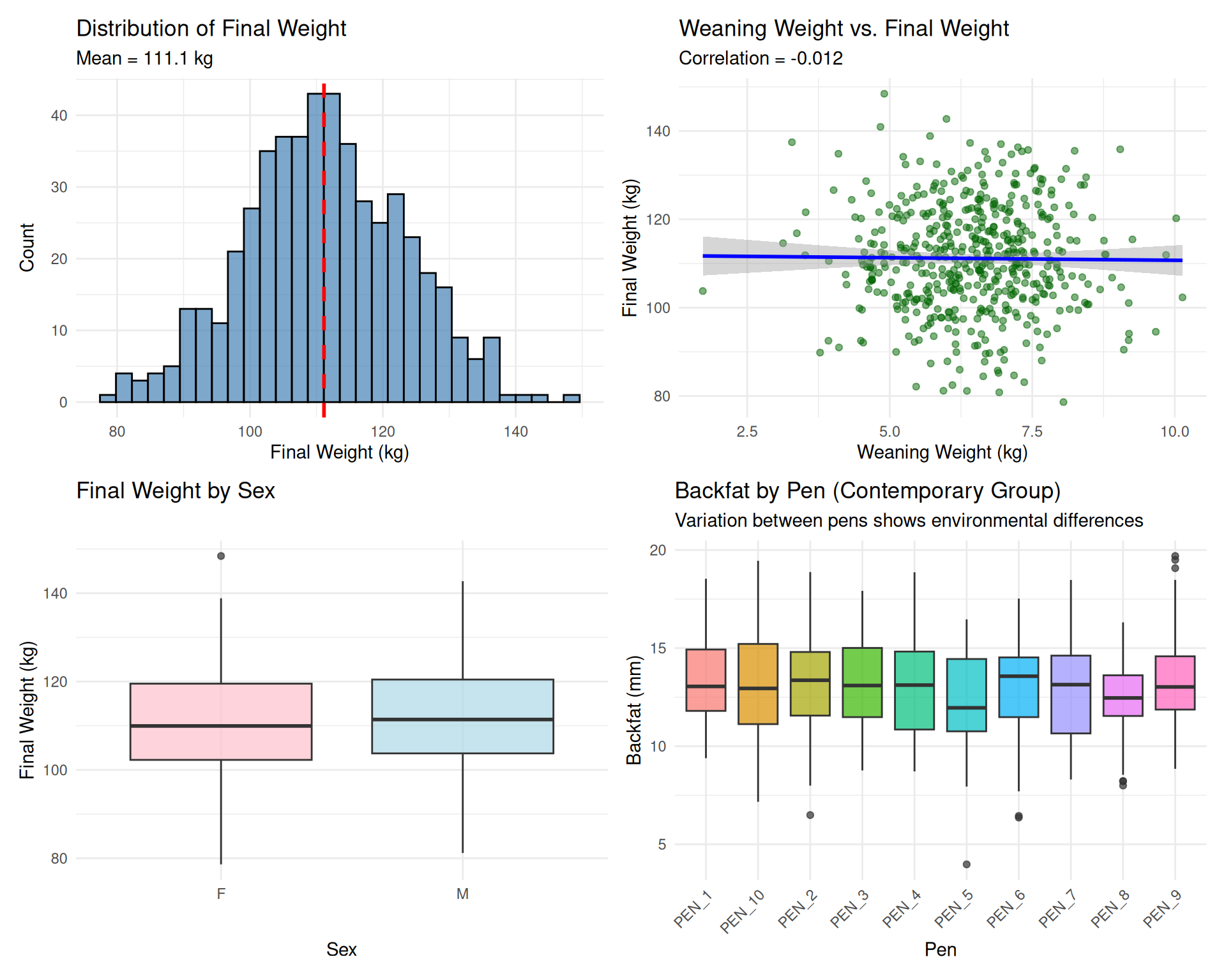
2.7.3 Demo 3: Outlier Detection
# Identify outliers using ±3 SD rule
detect_outliers <- function(data, trait) {
  mean_val <- mean(data[[trait]], na.rm = TRUE)
  sd_val <- sd(data[[trait]], na.rm = TRUE)

  lower_bound <- mean_val - 3 * sd_val
  upper_bound <- mean_val + 3 * sd_val

  outliers <- data %>%
    filter(.data[[trait]] < lower_bound | .data[[trait]] > upper_bound)

  cat("Outlier Detection for", trait, "\n")
  cat("Mean:", round(mean_val, 2), "\n")
  cat("SD:", round(sd_val, 2), "\n")
  cat("Range: [", round(lower_bound, 2), ",", round(upper_bound, 2), "]\n")
  cat("Number of outliers:", nrow(outliers), "\n\n")

  return(outliers)
}

# Check for outliers in final weight
outliers_weight <- detect_outliers(swine_data, "final_weight")
Outlier Detection for final_weight
Mean: 111.14
SD: 12.12
Range: [ 74.78 , 147.5 ]
Number of outliers: 1 # Check for outliers in backfat
outliers_backfat <- detect_outliers(swine_data, "backfat")Outlier Detection for backfat
Mean: 12.98
SD: 2.52
Range: [ 5.42 , 20.54 ]
Number of outliers: 1 # Visualize outliers
ggplot(swine_data, aes(x = final_weight, y = backfat)) +
geom_point(alpha = 0.5, color = "gray60") +
geom_point(data = outliers_weight, aes(x = final_weight, y = backfat),
color = "red", size = 3) +
geom_point(data = outliers_backfat, aes(x = final_weight, y = backfat),
color = "orange", size = 3) +
labs(title = "Outlier Detection: Final Weight and Backfat",
subtitle = "Red = final weight outliers, Orange = backfat outliers",
x = "Final Weight (kg)", y = "Backfat (mm)") +
theme_minimal()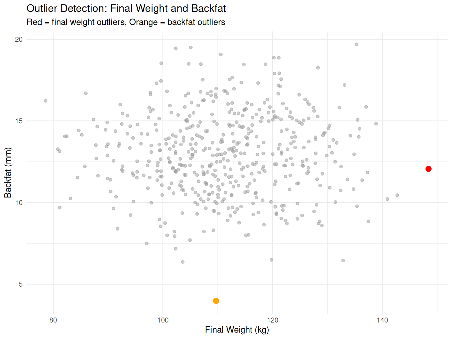
2.7.4 Demo 4: Contemporary Group Analysis
# Calculate means by contemporary group (pen)
cg_summary <- swine_data %>%
  group_by(pen) %>%
  summarise(
    n = n(),
    mean_final_weight = mean(final_weight),
    sd_final_weight = sd(final_weight),
    mean_backfat = mean(backfat),
    sd_backfat = sd(backfat),
    .groups = "drop"
  ) %>%
  arrange(desc(mean_final_weight))

print(cg_summary)
# A tibble: 10 × 6
pen n mean_final_weight sd_final_weight mean_backfat sd_backfat
<chr> <int> <dbl> <dbl> <dbl> <dbl>
1 PEN_7 58 114. 12.9 13.1 2.56
2 PEN_9 48 113. 12.5 13.3 2.63
3 PEN_1 37 113. 10.6 13.3 2.10
4 PEN_10 57 112. 9.84 13.1 2.84
5 PEN_6 50 111. 13.1 12.9 2.71
6 PEN_3 60 111. 12.3 13.2 2.36
7 PEN_8 52 111. 12.1 12.4 2.12
8 PEN_2 50 110. 12.6 13.2 2.59
9 PEN_4 44 108. 12.0 12.9 2.46
10 PEN_5 44 108. 12.6 12.2 2.61# Visualize contemporary group means
ggplot(cg_summary, aes(x = reorder(pen, mean_final_weight), y = mean_final_weight)) +
geom_col(fill = "steelblue", alpha = 0.7) +
geom_errorbar(aes(ymin = mean_final_weight - sd_final_weight,
ymax = mean_final_weight + sd_final_weight),
width = 0.3) +
labs(title = "Mean Final Weight by Pen (Contemporary Group)",
subtitle = "Error bars show ±1 SD. Environmental differences are substantial!",
x = "Pen", y = "Mean Final Weight (kg)") +
theme_minimal() +
theme(axis.text.x = element_text(angle = 45, hjust = 1))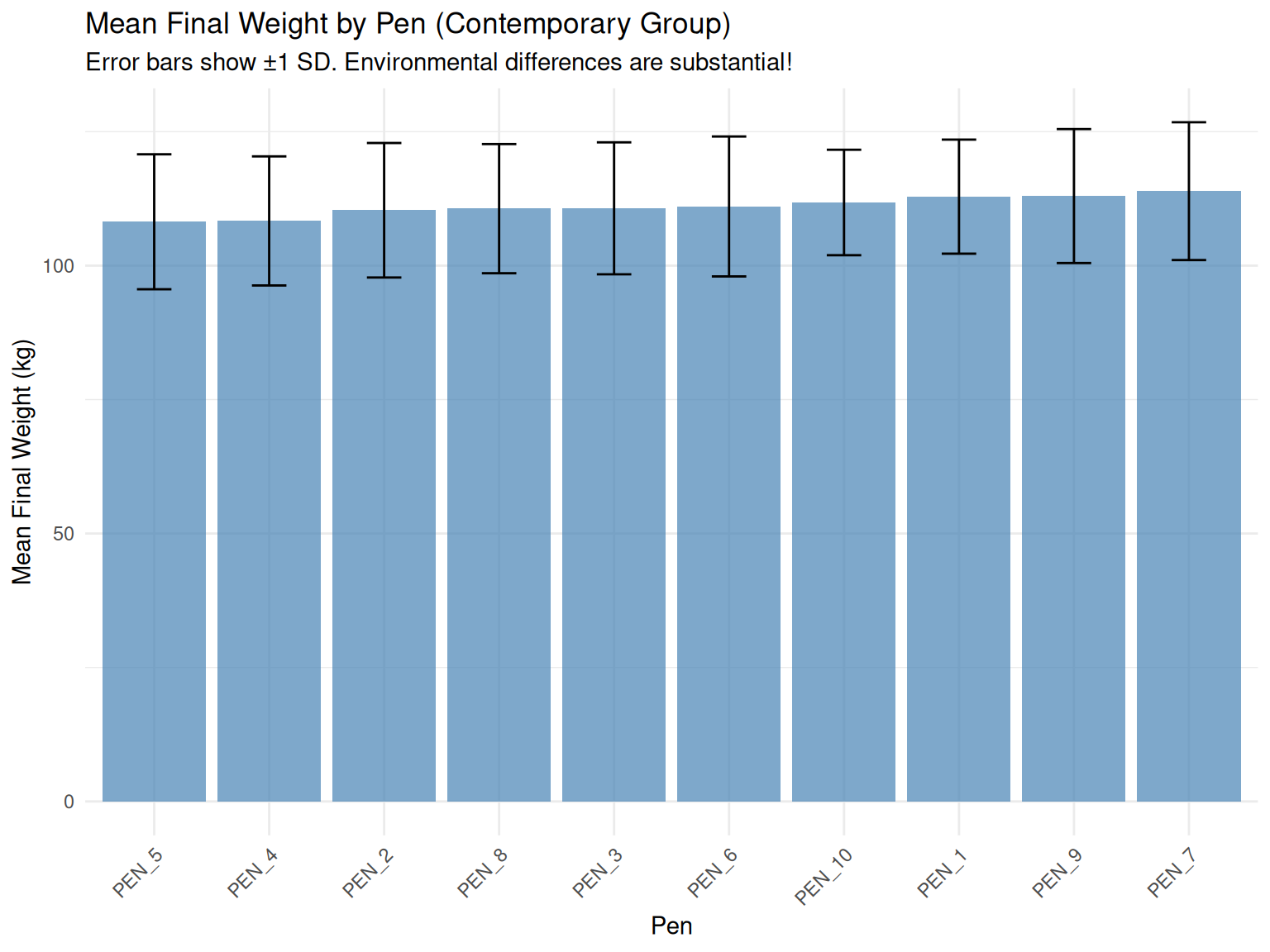
What Do These Demonstrations Show?
Demo 1: Real breeding programs have structured data (animals, pedigrees, phenotypes). Summary statistics help verify data quality.
Demo 2: Visualizing data reveals relationships (correlations), distributions (normality), and group effects (contemporary groups).
Demo 3: Outlier detection is critical for data quality control. Outliers may be real extremes or errors—investigate!
Demo 4: Contemporary group effects (pen, herd, year) create substantial environmental variation. Genetic evaluations must account for these effects to accurately estimate TBV.
2.8 Summary
This chapter laid the foundation for understanding what we select for in animal breeding and how we measure it. Let’s review the key concepts:
2.8.1 Key Points
1. Traits of Economic Importance
- Livestock traits fall into six categories: production, reproduction, health/fitness, efficiency, quality, and welfare
- High heritability traits (h² > 0.40) respond quickly to selection: growth rate, carcass traits, egg weight
- Low heritability traits (h² < 0.20) respond slowly: fertility, disease resistance, longevity
- Economic importance ≠ heritability — some low-heritability traits (e.g., fertility) have huge economic impact
2. Phenotypes and Phenotyping
- Phenotype = Genotype + Environment (P = G + E)
- High-quality phenotyping requires both accuracy (correct on average) and precision (repeatable)
- Challenges: Cost (electronic feeders $50K-100K+), time (longevity takes years), invasiveness (carcass traits require slaughter), throughput
- Modern technologies enable automated, high-throughput phenotyping: RFID feeders, milking robots, ultrasound, computer vision
3. Recording and Managing Data
- Animal identification is essential: Visual ID (ear tags), electronic ID (RFID), DNA parentage verification
- Data quality control prevents errors: Range checks, outlier detection, duplicate removal
- Validation rules catch errors at entry: Impossible dates, out-of-range values, missing required fields
- Relational databases organize data: Animals, Phenotypes, Genotypes tables linked by IDs
4. Breeding Objectives
- Breeding objective (H) defines what traits to improve and their relative economic importance
- Economic weights (v) quantify the value of one-unit genetic improvement in each trait
- Single-trait selection is fast but ignores correlated traits and can cause problems
- Multi-trait selection (selection index) balances multiple traits, accounting for economic values and genetic correlations
- Objectives differ by species and production role: Maternal vs. terminal (swine, beef), milk vs. beef (cattle)
5. True Breeding Value (TBV)
- TBV is the sum of average effects of an animal’s alleles—its genetic merit as a parent
- TBV is heritable: Animals pass (on average) half their TBV to each offspring
- TBV is unknown: We can never observe TBV directly, only phenotypes (P = TBV + E)
- EBVs are estimates of TBV: Combining own phenotype, relatives, pedigree, and genomic data using BLUP
- Goal of selection: Rank animals by TBV (or EBV) and select the top individuals as parents
The Foundation of Genetic Improvement
High-quality phenotypes + accurate data management + clear breeding objectives = successful genetic improvement.
Without accurate phenotypes, genetic evaluations will be biased. Without good data management, phenotypes will be unreliable or unusable. Without clear breeding objectives, we won’t know what traits to improve or how to weight them.
This chapter’s concepts underpin everything that follows in this course.
2.9 Practice Problems
2.9.1 Conceptual Questions
1. Trait Classification
Classify each of the following traits into one of the six categories (production, reproduction, health/fitness, efficiency, quality, welfare). Then indicate whether you expect the trait to have high (h² > 0.40), moderate (h² = 0.20-0.40), or low (h² < 0.20) heritability.
- Marbling score in beef cattle
- Litter size in swine
- Feed conversion ratio in broilers
- Somatic cell count (mastitis indicator) in dairy
- Egg shell strength in layers
- Temperament (docility) in beef cattle
2. Phenotype vs. TBV
Two Holstein cows, Bessie and Daisy, both produce 11,500 kg of milk in their first lactation.
- Bessie has an EBV of +400 kg for milk yield
- Daisy has an EBV of +800 kg for milk yield
- Why might both cows have the same phenotype (11,500 kg) despite different EBVs?
- Which cow would you prefer as a breeding animal? Why?
- If both cows are bred to the same bull (EBV = +600 kg), what is the expected milk yield of their daughters (assuming population average = 10,000 kg)?
3. Measurement Accuracy vs. Precision
Explain the difference between accuracy and precision in phenotypic measurements. Provide an example of a measurement that could be:
- Accurate but imprecise
- Precise but inaccurate
- Both accurate and precise
Why does each property matter for genetic evaluation?
4. Data Quality Control
You are reviewing weaning weight data for 100 piglets born in the same week. The mean weaning weight (21 days) is 6.2 kg with a standard deviation of 0.9 kg. Using the ±3 SD rule, you identify the following potential outliers:
- Piglet A: 12.5 kg
- Piglet B: 3.0 kg
- Piglet C: 9.1 kg
- For each piglet, calculate whether it falls outside the ±3 SD range.
- For each outlier, suggest two possible explanations (one biological, one data entry error).
- How would you investigate to determine if the value is correct or an error?
5. Breeding Objectives
Explain why a swine breeding company maintains separate breeding objectives for maternal lines (Large White, Landrace) vs. terminal sire lines (Duroc, Pietrain). What traits are emphasized in each, and why?
6. Contemporary Groups
Why is it important to account for contemporary group effects (e.g., pen, herd-year-season) when estimating breeding values? Provide an example showing how ignoring contemporary groups could lead to incorrect selection decisions.
2.9.2 Quantitative Problems
7. Heritability and Response
Backfat depth in swine has a heritability of h² = 0.50, a phenotypic mean of 13 mm, and a phenotypic standard deviation of 2.5 mm.
- If you select pigs with an average backfat of 10 mm as parents (3 mm below the mean), what is the expected selection differential (S)?
- What is the additive genetic standard deviation (σ_A)?
- Using the simplified formula R = h² × S, what is the expected response to selection in the offspring generation?
8. Economic Weights
A swine breeding program estimates the following economic weights for a terminal sire index:
- Average daily gain (ADG): +$15 per 100 g/day improvement
- Residual feed intake (RFI): -$30 per 0.1 kg/day improvement (negative RFI is better)
- Backfat depth: -$8 per 1 mm reduction
Two candidate boars have the following EBVs:
| Boar | ADG (g/day) | RFI (kg/day) | Backfat (mm) |
|---|---|---|---|
| Boar A | +50 | -0.15 | -1.0 |
| Boar B | +30 | -0.25 | -1.5 |
- Calculate the index value (H) for each boar.
- Which boar has superior genetic merit according to the index?
- Explain how genetic correlations between traits could influence which traits receive higher emphasis in the index (concept only, no calculations needed).
9. Outlier Detection in R
Using the swine_data dataset from Demo 1 in this chapter, write R code to:
- Calculate the mean and standard deviation of
weaning_weight - Identify all animals with weaning_weight values outside the ±3 SD range
- Create a histogram of weaning_weight with vertical lines showing the ±3 SD cutoffs
(Hint: Adapt the code from Demo 3.)
10. True Breeding Value Simulation
In the TBV conceptual diagram (Figure 6.5), we simulated a population where:
- TBV ~ N(100, 10²)
- Environment ~ N(0, 15²)
- Phenotype = TBV + Environment
- What is the heritability (h²) of this simulated trait? (Hint: h² = σ²_A / σ²_P, where σ²_A = σ²_TBV and σ²_P = σ²_TBV + σ²_E)
- If we select the top 20 animals by phenotype, would they also be the top 20 by TBV? Why or why not?
- Modify the simulation code to increase the heritability to h² = 0.80 (keeping σ²_TBV = 100). What must σ²_E be?
2.10 Further Reading
2.10.1 Textbooks and Reviews
-
Bourdon, R.M. (2000). Understanding Animal Breeding, 2nd ed. Prentice Hall.
- Chapters 2-4: Traits, phenotypes, breeding objectives
-
Falconer, D.S., and Mackay, T.F.C. (1996). Introduction to Quantitative Genetics, 4th ed. Longman.
- Chapter 1: The resemblance between relatives
- Chapter 10: Heritability
- Chapter 19: Selection: basic theory
-
Van Vleck, L.D., Pollak, E.J., and Oltenacu, E.A.B. (1987). Genetics for the Animal Sciences. W.H. Freeman.
- Chapter 3: Genetic and environmental variance
2.10.2 Industry Resources
-
National Swine Improvement Federation (NSIF): nsif.com
- Guidelines for phenotyping, data recording, and genetic evaluation in swine
-
Beef Improvement Federation (BIF): beefimprovement.org
- Guidelines for performance testing, contemporary groups, and EPDs
-
Council on Dairy Cattle Breeding (CDCB): uscdcb.com
- Information on trait definitions, genetic evaluations, and economic indices (Net Merit)
2.10.3 Scientific Papers
Phenotyping Technologies:
Halachmi, I., et al. (2019). Smart animal agriculture: Application of real-time sensors to improve animal well-being and production. Annual Review of Animal Biosciences 7:403-425.
Matthews, S.G., et al. (2016). Early detection of health and welfare compromises through automated detection of behavioural changes in pigs. The Veterinary Journal 217:43-51.
Breeding Objectives and Economic Weights:
Groen, A.F., et al. (1997). Economic values in dairy cattle breeding, with special reference to functional traits. Report on an EAAP-working group. Livestock Production Science 49:1-21.
VanRaden, P.M., and Multi-State Project S-1040. (2004). Invited review: Selection on net merit to improve lifetime profit. Journal of Dairy Science 87:3125-3131.
Data Quality and Management:
- Berry, D.P., et al. (2011). Imputation of genotypes from low- to high-density genotyping platforms and implications for genomic selection. Animal 5:1162-1169. (Discusses data quality in genomics context)
2.10.4 Online Tools and Databases
-
Animal QTLdb: animalgenome.org/cgi-bin/QTLdb
- Database of quantitative trait loci (QTL) and their effects on livestock traits
-
USDA AIPL Genetic Evaluations: aipl.arsusda.gov
- Dairy cattle genetic evaluations, trend data, and documentation
Looking Ahead
In Chapter 3, we’ll formalize the genetic model introduced in this chapter. We’ll partition the genetic component into additive, dominance, and epistatic effects, and derive the fundamental equation:
\[P = \mu + A + D + I + E\]
This will set the stage for understanding heritability (Chapter 5), breeding value estimation (Chapter 7), and ultimately selection response (Chapter 6).
The journey into quantitative genetics continues!