Explain the principles and advantages of genomic selection
Distinguish GBLUP, SNP-BLUP, and Bayesian genomic prediction methods
Understand single-step genomic BLUP and its practical importance
Describe how genomic selection has impacted livestock breeding
Calculate expected accuracy of genomic predictions
13.1 Introduction
In 2001, Theo Meuwissen, Ben Hayes, and Mike Goddard published a paper that would fundamentally change animal breeding. Titled “Prediction of Total Genetic Value Using Genome-Wide Dense Marker Maps,” this landmark paper proposed something revolutionary: What if we could predict an animal’s breeding value directly from its DNA, without waiting for performance records or progeny data?
At the time, this seemed almost too good to be true. Traditional animal breeding relied heavily on performance testing and progeny trials, which took years to complete. A dairy bull, for example, needed 5-6 years of progeny testing before breeders could confidently estimate his genetic merit for milk production. By the time his breeding value was known, he might be past his prime reproductive years. The same challenges existed across all livestock species—genetic evaluation was accurate but slow.
Meuwissen and colleagues proposed using thousands of DNA markers (SNPs) spread across the entire genome to capture the effects of all genes affecting a trait. Because these markers are in linkage disequilibrium with the actual causal mutations, they could “tag” the genetic variation responsible for differences in performance. With a large enough training population of animals with both genotypes and phenotypes, one could estimate the relationship between SNP patterns and breeding values. These estimated relationships could then be applied to young animals with only genotype data, providing accurate predictions at birth—or even as embryos.
The impact of this idea has been nothing short of transformative. Dairy cattle breeding adopted genomic selection in 2009, and the rate of genetic improvement immediately doubled. Similar revolutions followed in swine (2011-2014), poultry (2010-2015), and beef cattle (2012-2017). Today, genomic selection is the standard approach in nearly all major breeding programs worldwide.
This chapter explains how genomic selection works. In Chapter 12, we learned about SNPs, genotyping technologies, and data quality control—the raw materials of genomic selection. Now we’ll explore the statistical methods that turn genotype data into genomic predictions. We’ll cover three major approaches:
GBLUP (Genomic BLUP): Uses a genomic relationship matrix to predict breeding values
Bayesian methods: Allows different SNPs to have different effect sizes
Single-step GBLUP: Combines pedigree and genomic information in one unified analysis
By the end of this chapter, you’ll understand why genomic selection has revolutionized animal breeding, and how breeding companies use these methods to accelerate genetic progress.
13.2 What is Genomic Selection?
Genomic selection is a method of predicting an animal’s breeding value using genome-wide SNP genotype data. The predicted value is called a GEBV (Genomic Estimated Breeding Value), which represents our best estimate of an animal’s true breeding value based on its DNA sequence.
The fundamental idea is elegantly simple:
Build a training population: Collect genotype and phenotype data (or conventional EBVs) on thousands of animals
Estimate the relationship: Use statistical models to learn how SNP patterns relate to breeding values
Predict for selection candidates: Apply the learned relationships to young, genotyped animals who don’t yet have their own performance records
Select the best: Choose parents based on GEBVs instead of waiting for performance or progeny data
This approach breaks the traditional trade-off between accuracy and generation interval that constrained animal breeding for decades.
13.2.1 Traditional Selection (Pre-Genomics)
Before genomics, breeders faced a fundamental challenge: accurate genetic evaluation required time.
For a young dairy bull with no daughters yet, the only information available was his pedigree. His estimated breeding value was essentially the average of his parents’ EBVs—what we call the parent average or pedigree index. The accuracy of this prediction was modest at best:
Accuracy for young animals: r ≈ 0.30-0.40 (based on parent average only)
Selection intensity: Limited, because predictions were imprecise
To improve accuracy, breeders used progeny testing: mate the young bull to many cows, wait for daughters to lactate, measure their milk production, and calculate the bull’s EBV based on daughter performance. This worked well for accuracy:
Accuracy with progeny data: r ≈ 0.85-0.90 (after 50-100 daughters with records)
But progeny testing came at a steep cost:
Generation interval: 5-7 years (birth → mating → daughters born → daughters mature → milk records collected → EBV computed)
Expense: $25,000-$50,000 per bull (semen storage, matings, data collection)
Opportunity cost: By the time a bull’s genetic merit was known, newer genetics might already be available
This same pattern held across species. In swine, boars needed progeny in multiple litters before feed efficiency could be accurately evaluated. In beef cattle, carcass merit could only be assessed after offspring were slaughtered. The fundamental constraint was always the same: accuracy required waiting for phenotypes, which meant long generation intervals and slow genetic progress.
13.2.2 Genomic Selection
Genomic selection changes everything by providing moderate to high accuracy at birth, without waiting for performance or progeny records.
Here’s what genomic selection uses:
Training population: Animals with both genotypes and phenotypes (or traditional EBVs)
Dairy: Thousands of progeny-tested bulls with daughter records
Swine: Thousands of pigs with growth, carcass, and reproduction records
Poultry: Tens of thousands of birds with production records
Genomic prediction model: Statistical method that learns how SNP patterns correlate with breeding values (more on this below)
Selection candidates: Young animals with genotypes but no performance records
The result:
Accuracy for young animals: r ≈ 0.50-0.70 (depending on training population size, heritability, and relationships)
At birth (or even as embryos): No need to wait for maturity or progeny
Generation interval: Cut in half or more
Dairy: From 6-7 years → 2.5-3 years
Swine: From 1.8 years → 1.0-1.2 years
The key advantage is not just accuracy—it’s high accuracy with short generation interval. Recall the breeder’s equation from Chapter 6:
\[R = \frac{i \times r \times \sigma_A}{L}\]
Genomic selection improves both numerator (r increases for young animals) and denominator (L decreases because we don’t need to wait for progeny). The combined effect on genetic progress is dramatic: in U.S. dairy cattle, annual genetic gain for milk yield doubled from ~120 kg/year to ~250 kg/year after genomic selection was adopted in 2009.
13.3 Why Genomic Selection Works
To understand why genomic selection works, we need to recall a fundamental principle from Chapter 12: SNPs are not usually the causal mutations that directly affect traits. Instead, they serve as markers that are statistically associated with nearby causal mutations. This association, called linkage disequilibrium, is the genetic foundation of genomic prediction.
13.3.1 Linkage Disequilibrium (LD)
Linkage disequilibrium (LD) is the non-random association of alleles at different loci. When two loci are in LD, knowing the allele at one locus tells you something about the likely allele at the other locus.
LD exists for several reasons:
Physical proximity: Loci close together on the same chromosome are less likely to be separated by recombination
Recent mutation: Newly arisen mutations haven’t had time to recombine onto different genetic backgrounds
Population history: Genetic drift, population bottlenecks, and selection create LD patterns
Limited recombination: Even over many generations, recombination is a relatively slow process
Here’s the key insight: If a SNP is in LD with a causal mutation (sometimes called a QTN—Quantitative Trait Nucleotide), then animals with a particular SNP allele will tend to have a particular QTN allele. The SNP “tags” the causal variant.
For example, imagine a causal mutation that increases milk production by 50 kg per lactation. A nearby SNP might be in strong LD with this mutation. Even though the SNP itself doesn’t affect milk yield, animals with the “A” allele at the SNP position will tend to carry the beneficial allele at the causal mutation. By tracking the SNP allele, we indirectly track the causal allele.
The strength of LD decays with physical distance. In cattle, SNPs separated by 50,000 base pairs (50 kb) might have moderate LD, while SNPs 1 million base pairs apart typically have little LD. This is why dense SNP panels (50K or 600K+ SNPs) are necessary—we need enough markers to ensure that most causal mutations are in LD with at least one SNP on the array.
13.3.2 Capturing Additive Genetic Variance
Quantitative traits like milk production, growth rate, and litter size are affected by hundreds to thousands of genes scattered across the genome. Each gene contributes a small amount to the total genetic variance. Genomic selection doesn’t require identifying every causal gene—it just needs enough SNPs in LD with enough causal loci to capture most of the additive genetic variance.
With a 50K SNP panel (one SNP every ~50,000 base pairs on average), we have excellent genome coverage in most livestock species. Even if we don’t know which SNPs are causal, the combination of all SNP effects will track the sum of nearby causal effects. This “polygenic” approach works remarkably well for complex traits.
The proportion of additive genetic variance captured depends on:
Poultry: N_e ≈ 50-100, longer LD (easier to capture variance)
Recombination rate: Varies across chromosomes and species
In practice, 50K SNP arrays capture 70-90% of additive genetic variance for most traits in dairy cattle. Higher-density arrays (600K+) capture slightly more, but the gain is modest. This is good news: we don’t need perfect genome coverage, just good coverage.
13.3.3 Training Population
The training population (also called the reference population) is the cornerstone of genomic selection. These are animals with:
Genotypes: SNP data from a chip or sequencing
Phenotypes: Performance records, or conventional EBVs based on their own and relatives’ records
The training population is used to “train” the genomic prediction model—that is, to estimate how SNP patterns relate to breeding values. The larger and more representative the training population, the more accurate the genomic predictions will be.
Key factors for an effective training population:
Size: Larger is better. Thousands of animals are typically needed for moderate to high accuracy
Dairy: 10,000-50,000 bulls with progeny-tested EBVs
Swine: 5,000-20,000 pigs with performance records
Poultry: 20,000-100,000 birds (huge populations possible due to low genotyping costs)
Relationship to selection candidates: Predictions are most accurate for animals closely related to the training population
Ideally, training population includes sires, dams, and close relatives of candidates
Accuracy declines if training and selection populations are distantly related (e.g., different breeds)
Phenotype quality: Accurate, well-recorded phenotypes lead to better predictions
Training on progeny-tested EBVs (high accuracy) is better than training on single records
Updated regularly: As new data become available, re-train the model to maintain accuracy
Once the training population is established and the model is trained, we can predict GEBVs for any genotyped animal—even newborns with no performance records. This is the power of genomic selection: the training population does the “heavy lifting” of connecting genotypes to phenotypes, and selection candidates benefit from this accumulated knowledge.
13.4 Two Main Approaches to Genomic Prediction
There are two philosophical frameworks for genomic prediction, which differ in what they estimate:
Animal model approach (also called “breeding value model”): Estimate breeding values directly for each animal, using genomic relationships
Marker effects model: Estimate the effect of each SNP, then sum SNP effects to calculate breeding values
These approaches sound fundamentally different, but mathematically they are often equivalent—they’re just different ways of parameterizing the same underlying model. However, they differ in computational approach, interpretation, and practical application.
13.4.1 Animal Model Approach (GBLUP)
In the animal model approach, we estimate breeding values directly, just as in traditional BLUP (Chapter 7). The key difference is that we replace the pedigree relationship matrix (A) with the genomic relationship matrix (G).
What we estimate: Breeding values (u) for each animal
Model: \[y = X\beta + Zu + e\]
Where:
y = phenotypes (or EBVs from traditional evaluation)
X = design matrix for fixed effects (contemporary groups, etc.)
β = vector of fixed effects
Z = design matrix relating animals to records
u = vector of breeding values (random effects)
e = residual errors
The key difference from traditional BLUP: breeding values are assumed to follow:
\[u \sim N(0, G\sigma^2_u)\]
That is, breeding values have a covariance structure defined by the genomic relationship matrix G (not the pedigree relationship matrix A).
Advantages:
Conceptually simple (same framework as traditional BLUP)
G captures realized relationships (Mendelian sampling)
Efficient computation for large datasets
Most widely used in practice
This approach is called GBLUP (Genomic BLUP).
13.4.2 Marker Effects Model Approach
In the marker effects model approach, we estimate the effect of each individual SNP, then sum those effects to calculate breeding values.
What we estimate: SNP effects (β_j) for each of thousands of SNPs
Methods in this category include SNP-BLUP (assumes all SNPs have equal variance) and Bayesian methods (allow SNPs to have different variances).
13.4.3 Equivalence of GBLUP and SNP-BLUP
Under certain assumptions, GBLUP (animal model) and SNP-BLUP (marker effects model) are mathematically equivalent—they produce identical GEBVs.
Specifically, when:
All SNPs have equal variance (no large-effect QTL)
The genomic relationship matrix G is computed as: \(G = \frac{MM'}{2\sum p_j(1-p_j)}\) (VanRaden’s first method)
Then the breeding values from GBLUP equal the sum of SNP effects from SNP-BLUP.
This equivalence is powerful: we can choose whichever approach is computationally convenient. For large datasets with many animals, GBLUP is often faster. For datasets with more SNPs than animals, SNP-BLUP may be more efficient.
13.4.4 Practical Differences
Despite mathematical equivalence, the two approaches differ in practice:
Feature
Animal Model (GBLUP)
Marker Effects Model (SNP-BLUP, Bayesian)
Estimates
Breeding values (u)
SNP effects (β)
Computation
Fast for large n
Faster for large m
Interpretation
Directly provides GEBVs
Provides SNP effects; sum to get GEBVs
SNP information
Implicit (via G matrix)
Explicit (each SNP has estimated effect)
Flexibility
Less flexible (assumes equal variance)
More flexible (can vary SNP variances)
Software
ASReml, BLUPF90
BGLR, GenSel, brms
Use case
Standard industry practice
Research, QTL mapping, traits with major genes
In the following sections, we’ll explore GBLUP, SNP-BLUP, and Bayesian methods in detail.
13.5 GBLUP (Genomic BLUP)
GBLUP (Genomic Best Linear Unbiased Prediction) is the animal model approach to genomic selection. It extends traditional BLUP (Chapter 7) by replacing the pedigree relationship matrix (A) with a genomic relationship matrix (G) that captures the actual realized relationships between animals based on their DNA.
GBLUP was popularized by Paul VanRaden’s 2008 paper “Efficient Methods to Compute Genomic Predictions,” which provided computationally feasible methods for calculating G and solving genomic evaluations. Today, GBLUP is the foundation of genomic selection in dairy cattle, beef cattle, and many other species.
13.5.1 Genomic Relationship Matrix (G)
The genomic relationship matrix (G) quantifies the genetic similarity between pairs of animals based on their SNP genotypes. It’s analogous to the pedigree relationship matrix (A), but instead of relying on expected relationships from the pedigree, G uses the realized (actual) sharing of genome segments.
Key differences between A and G:
Feature
A (Pedigree Matrix)
G (Genomic Matrix)
Based on
Pedigree records
SNP genotypes
Relationship
Expected (average)
Realized (actual)
Full-sibs
Always 0.50
Varies (e.g., 0.47-0.53)
Mendelian sampling
Not captured
Captured
Unknown pedigree
Cannot calculate
Can still calculate
Self-relationship
1.0 or 1 + F
Close to 1.0 (with adjustments)
The beauty of G is that it captures Mendelian sampling—the random variation in which parental alleles are inherited by offspring. Even full-siblings don’t share exactly 50% of their genome; some pairs share 48%, others 52%, due to random segregation and recombination. G captures this variation, making predictions more accurate.
13.5.2 Calculating G: VanRaden’s Method
Paul VanRaden (2008) proposed an efficient method for computing G from SNP genotypes. The formula is:
Important note: You don’t need to solve MMEs by hand! Software packages (ASReml, BLUPF90, etc.) do this for you. The key concept is that GBLUP uses G instead of A, and this improves accuracy because G captures realized relationships.
13.5.4 Advantages of GBLUP
Captures Mendelian sampling: G reflects actual genome sharing, not just expected relationships
High accuracy for young animals: Animals with genotypes but no phenotypes can receive accurate GEBVs (r = 0.50-0.70) based on realized relationships with the training population
Works with incomplete pedigrees: G can be calculated even if pedigree is unknown (as long as genotypes are available)
Computationally efficient: For large datasets (n > 10,000), GBLUP is faster than marker effects models
Widely implemented: Standard method in dairy, beef, swine, poultry
13.5.5 Numerical Example: Calculating G
Let’s calculate the genomic relationship matrix for 5 animals genotyped at 6 SNPs (in reality, we’d use 50,000+ SNPs, but the principle is the same).
Step 1: Genotype data (M)
Animal
SNP1
SNP2
SNP3
SNP4
SNP5
SNP6
1
2
1
0
2
1
1
2
1
2
1
1
0
2
3
0
0
2
0
2
0
4
2
1
1
2
1
1
5
1
1
0
1
2
2
Step 2: Calculate allele frequencies (p_j)
For SNP1: p_1 = (2+1+0+2+1) / (2×5) = 6/10 = 0.60
Similarly:
p_2 = 0.50
p_3 = 0.40
p_4 = 0.60
p_5 = 0.60
p_6 = 0.60
Step 3: Create P matrix (expected genotypes)
P has the same dimensions as M, but every element in column j is \(2p_j\):
Animal
SNP1
SNP2
SNP3
SNP4
SNP5
SNP6
1
1.2
1.0
0.8
1.2
1.2
1.2
2
1.2
1.0
0.8
1.2
1.2
1.2
3
1.2
1.0
0.8
1.2
1.2
1.2
4
1.2
1.0
0.8
1.2
1.2
1.2
5
1.2
1.0
0.8
1.2
1.2
1.2
Step 4: Compute (M - P) (centered genotypes)
Animal
SNP1
SNP2
SNP3
SNP4
SNP5
SNP6
1
0.8
0.0
-0.8
0.8
-0.2
-0.2
2
-0.2
1.0
0.2
-0.2
-1.2
0.8
3
-1.2
-1.0
1.2
-1.2
0.8
-1.2
4
0.8
0.0
0.2
0.8
-0.2
-0.2
5
-0.2
0.0
-0.8
-0.2
0.8
0.8
Step 5: Compute \((M-P)(M-P)'\)
This is a 5×5 matrix. For example, element (1,1) is: \[(0.8)^2 + (0.0)^2 + (-0.8)^2 + (0.8)^2 + (-0.2)^2 + (-0.2)^2 = 0.64 + 0 + 0.64 + 0.64 + 0.04 + 0.04 = 2.00\]
# Step 1: Calculate allele frequencies from the data# (In practice, these might be from a larger reference population)p_j<-colMeans(M)/2# Allele frequency at each SNPcat("\nFirst 10 allele frequencies:\n")
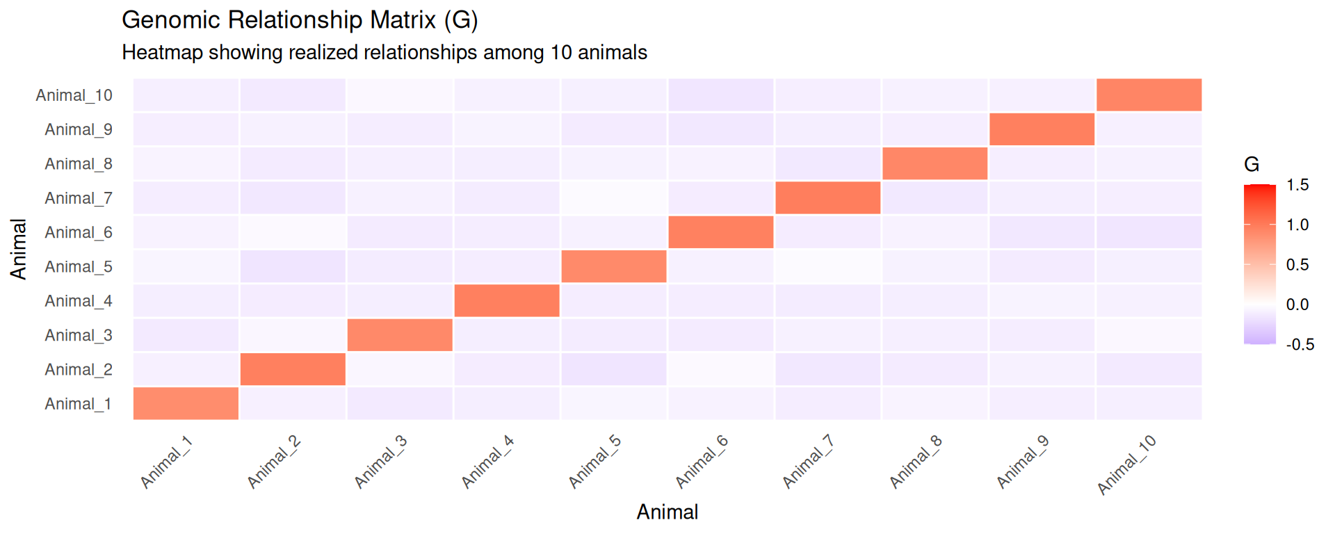
# Visualize G matrix as heatmapG_melted<-melt(G)colnames(G_melted)<-c("Animal_1", "Animal_2", "Relationship")p1<-ggplot(G_melted, aes(x =Animal_1, y =Animal_2, fill =Relationship))+geom_tile(color ="white", linewidth =0.5)+scale_fill_gradient2(low ="blue", mid ="white", high ="red", midpoint =0, limits =c(-0.5, 1.5), name ="G")+labs(title ="Genomic Relationship Matrix (G)", subtitle ="Heatmap showing realized relationships among 10 animals", x ="Animal", y ="Animal")+theme_minimal(base_size =11)+theme(axis.text.x =element_text(angle =45, hjust =1), panel.grid =element_blank())print(p1)
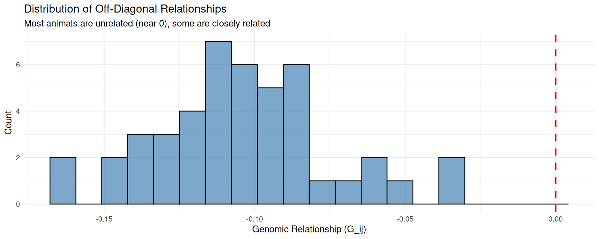
# Distribution of off-diagonal relationshipsp2<-ggplot(data.frame(Relationship =off_diag), aes(x =Relationship))+geom_histogram(bins =20, fill ="steelblue", color ="black", alpha =0.7)+geom_vline(xintercept =0, linetype ="dashed", color ="red", linewidth =1)+labs(title ="Distribution of Off-Diagonal Relationships", subtitle ="Most animals are unrelated (near 0), some are closely related", x ="Genomic Relationship (G_ij)", y ="Count")+theme_minimal(base_size =11)print(p2)
Key observations from the G matrix:
Diagonal elements average close to 1.0, indicating animals are as homozygous as expected on average
Off-diagonal elements show variation in relationships:
Values near 0 indicate unrelated animals
Positive values indicate animals share more alleles than average (related)
Negative values indicate animals have complementary allele sets (less related than random)
With 1000 SNPs, the G matrix estimates are reasonably stable, though more SNPs (50K+) would provide even better precision
This G matrix could now be used in GBLUP to estimate genomic breeding values for these animals.
13.6 SNP-BLUP and Marker Effects Models
While GBLUP estimates breeding values directly using the genomic relationship matrix, marker effects models estimate the effect of each individual SNP. This approach provides explicit information about which genomic regions contribute to genetic variation—useful for understanding the genetic architecture of traits and for identifying candidate genes.
13.6.1 SNP-BLUP
SNP-BLUP is the marker effects equivalent of GBLUP. Instead of estimating n breeding values (one per animal), we estimate m SNP effects (one per SNP, where m might be 50,000 or more).
Model:
\[y = X\alpha + M\beta + e\]
Where:
y = vector of phenotypes (n × 1)
X = design matrix for fixed effects
α = vector of fixed effects
M = centered genotype matrix (n × m), where M_ij = x_ij - 2p_j
β = vector of SNP effects (m × 1)
e = vector of residuals
Assumptions:
SNP effects are random: \(\beta_j \sim N(0, \sigma^2_\beta)\)
All SNPs have equal variance\(\sigma^2_\beta\)
This equal-variance assumption is key: SNP-BLUP treats all SNPs as contributing equally (on average) to genetic variation.
Estimating SNP effects: We solve for \(\hat{\beta}\) using ridge regression (penalized regression) or mixed model equations. The penalty shrinks small effects toward zero, preventing overfitting.
Computing GEBVs from SNP effects:
Once we have estimated SNP effects \(\hat{\beta}\), we calculate each animal’s GEBV by summing the contributions of all SNPs:
Animal A’s GEBV is +0.154 kg above the population mean for milk yield.
13.6.2 Equivalence of GBLUP and SNP-BLUP
Here’s a remarkable mathematical result: Under certain conditions, GBLUP and SNP-BLUP produce identical GEBVs. They are different parameterizations of the same underlying model.
When they are equivalent:
All SNPs have equal variance (the SNP-BLUP assumption)
The genomic relationship matrix is computed as \(G = \frac{MM'}{2\sum p_j(1-p_j)}\) (VanRaden’s method)
Under these conditions:
\[GEBV_{GBLUP} = GEBV_{SNP-BLUP}\]
Why this equivalence matters:
Computational flexibility: Choose the approach that’s faster for your dataset
GBLUP: Faster when n (animals) < m (SNPs)—invert an n × n matrix (G) instead of solving m equations
SNP-BLUP: Faster when m < n (rare in livestock, but possible with low-density panels)
Interpretability: SNP-BLUP provides explicit SNP effects (useful for genomic architecture studies), while GBLUP is a “black box”
Extensions: SNP-BLUP framework allows relaxing the equal-variance assumption (Bayesian methods)
Mathematical connection:
The relationship between breeding values (u) and SNP effects (β) is:
\[u = M\beta\]
And:
\[G = \frac{MM'}{2\sum p_j(1-p_j)} \propto MM'\]
So breeding values are linear combinations of SNP effects, and genomic relationships are determined by the similarity of SNP genotype patterns.
13.6.3 When to Use SNP-BLUP vs. GBLUP
Situation
Best Approach
Reason
Standard genomic evaluation (50K SNPs, 10,000+ animals)
GBLUP
Faster computation
Identifying important genomic regions
SNP-BLUP
Provides explicit SNP effects
Traits with major QTL
Bayesian methods (next section)
Allows unequal SNP variances
Integrating genotyped and non-genotyped animals
Single-step GBLUP (discussed later)
Handles both efficiently
Research on genetic architecture
SNP-BLUP or Bayesian
Interpretable SNP effects
In practice, GBLUP dominates in industry because it’s computationally efficient and easy to implement in existing BLUP software. SNP-BLUP and Bayesian methods are more common in research and for specific applications where understanding SNP effects is important.
13.7 Bayesian Methods
Both GBLUP and SNP-BLUP assume that all SNPs contribute equally (on average) to genetic variance. This is a reasonable first approximation for many traits, but it’s not realistic for all traits. Some traits are influenced by a few large-effect QTL, while most SNPs have little to no effect. Bayesian methods relax the equal-variance assumption and allow SNPs to have different effect sizes—or even zero effect.
13.7.1 Motivation
The equal-variance assumption of SNP-BLUP implies that the genetic architecture is infinitesimal: thousands of genes each contributing tiny, equal effects. This assumption works well for traits like body weight or milk yield, which are truly polygenic.
However, consider these examples where the infinitesimal assumption breaks down:
Milk fat percentage in dairy cattle: The DGAT1 gene explains ~30% of genetic variance—one gene with a huge effect
Coat color: A few major genes (MC1R, KIT, etc.) determine most variation
Polled/horned in cattle: The POLLED gene has a near-Mendelian effect
Disease resistance: Some pathogens have major resistance loci (e.g., MHC region)
For these traits, forcing all SNPs to have equal variance is inefficient. It would be better to estimate large effects for SNPs near major QTL and small (or zero) effects for SNPs in neutral regions.
This is exactly what Bayesian methods do: they use prior distributions that allow SNPs to have different variances, giving the model flexibility to identify major-effect loci while shrinking small effects toward zero.
13.7.2 The Bayesian Framework
In Bayesian statistics, we combine:
Prior distribution: Our beliefs about parameters before seeing data (e.g., “most SNPs have small effects”)
Likelihood: The probability of the data given parameters
Posterior distribution: Updated beliefs about parameters after seeing data
For genomic prediction, we specify a prior distribution for SNP effects (β) that reflects our belief about genetic architecture. The data then updates these priors, yielding a posterior distribution for SNP effects. We use Markov Chain Monte Carlo (MCMC) to sample from the posterior.
13.7.3 BayesA
BayesA was proposed by Meuwissen, Hayes, and Goddard (2001) as one of the original genomic selection methods.
Key idea: All SNPs have effects, but each SNP has its own variance.
\(S^2\) = scale parameter (related to expected genetic variance)
Interpretation:
Each SNP has its own variance (\(\sigma^2_{\beta_j}\))
The prior on \(\sigma^2_{\beta_j}\) has heavy tails, allowing some SNPs to have large variances (large effects)
Most SNPs will have small variances, but the model is flexible enough to accommodate a few large-effect SNPs
Result: SNPs near QTL get large effect estimates, while most SNPs get small (shrunken) estimates.
13.7.4 BayesB
BayesB extends BayesA by allowing some SNPs to have exactly zero effect.
Key idea: Only a proportion (\(\pi\)) of SNPs affect the trait; the rest have β_j = 0.
Model:
\[\beta_j = \begin{cases} 0 & \text{with probability } \pi \\ N(0, \sigma^2_{\beta_j}) & \text{with probability } 1-\pi \end{cases}\]
Where \(\sigma^2_{\beta_j}\) again follows a scaled inverse chi-square distribution (as in BayesA).
Interpretation:
This is a mixture prior: SNPs are either “in the model” (with non-zero effect) or “out of the model” (zero effect)
\(\pi\) is pre-specified (e.g., \(\pi = 0.95\) means 95% of SNPs have zero effect, 5% have non-zero effects)
SNPs in the model can have large effects (heavy-tailed prior on variance)
Result: The model performs variable selection—it identifies which SNPs are important and sets the rest to zero. This can improve accuracy for traits with few major QTL.
13.7.5 BayesC and BayesCπ
BayesC is similar to BayesB, but SNPs “in the model” all share the same variance (like SNP-BLUP), rather than having individual variances.
BayesCπ (BayesC-pi) extends BayesC by estimating \(\pi\) (the proportion of SNPs with zero effect) from the data, rather than pre-specifying it.
Key idea: Let the data tell us how many SNPs affect the trait.
Model:
\[\beta_j = \begin{cases} 0 & \text{with probability } \pi \\ N(0, \sigma^2_{\beta}) & \text{with probability } 1-\pi \end{cases}\]
Prior on \(\pi\):
\[\pi \sim \text{Uniform}(0, 1)\]
Or a more informative prior, e.g., Beta(1, 10), which favors most SNPs having zero effect.
Interpretation:
The model learns how “sparse” the genetic architecture is (i.e., what proportion of SNPs matter)
If the trait is highly polygenic, \(\pi\) will be estimated near 0 (few SNPs excluded)
If the trait is oligogenic (few QTL), \(\pi\) will be estimated near 1 (most SNPs excluded)
13.7.6 Bayesian Lasso
The Bayesian Lasso uses a double exponential (Laplace) prior on SNP effects:
This prior strongly shrinks small effects toward zero (like ridge regression but stronger)
Allows a few large effects to remain large
Does not perform explicit variable selection (all SNPs have non-zero effects, but many are tiny)
Computationally faster than BayesA/B/C
13.7.7 Comparing Bayesian Methods
Method
SNPs with β = 0?
Variance per SNP
Estimates \(\pi\)?
Best for…
BayesA
No
Individual \(\sigma^2_{\beta_j}\)
N/A
Moderate polygenicity, some large QTL
BayesB
Yes (π pre-specified)
Individual \(\sigma^2_{\beta_j}\)
No
Few large QTL, sparse architecture
BayesC
Yes (π pre-specified)
Shared \(\sigma^2_{\beta}\)
No
Few QTL, but equal-sized effects
BayesCπ
Yes (π estimated)
Shared \(\sigma^2_{\beta}\)
Yes
Unknown architecture, data decides
Bayesian Lasso
No
Regularized via λ
N/A
Fast computation, moderate sparsity
13.7.8 When Bayesian Methods Help
Bayesian methods can improve genomic prediction accuracy over GBLUP/SNP-BLUP, but the gain depends on the trait’s genetic architecture:
Large gains (5-15% higher accuracy):
Traits with a few major QTL (e.g., milk fat %, coat color, some disease resistance)
Oligogenic traits (controlled by 5-50 genes)
Modest gains (0-5% higher accuracy):
Moderately polygenic traits (e.g., milk yield, body weight)
Traits where most QTL have small effects, but a few are larger
Little or no gain (< 1% higher accuracy):
Highly polygenic traits with purely infinitesimal architecture
Traits with very low heritability (limited signal to detect QTL)
Trade-off: Bayesian methods are computationally expensive. MCMC requires thousands of iterations, and each iteration updates thousands of SNP effects. For large datasets (50K SNPs, 10,000 animals), Bayesian methods may take hours to days, while GBLUP takes minutes.
13.7.9 Software for Bayesian Genomic Prediction
Software
Methods
Platform
Notes
BGLR
BayesA, BayesB, BayesC, Bayesian Lasso, more
R
Most popular R package, well-documented
GenSel
BayesB, BayesCπ
Standalone (Fortran)
Developed by Rohan Fernando’s group (Iowa State)
bayz
Flexible Bayesian models
R
General Bayesian modeling for genetics
JWAS
Bayesian methods + single-step
Julia
Fast, modern language
Example using BGLR (conceptual):
library(BGLR)# y = phenotypes, M = genotype matrixfit_BayesB<-BGLR(y =y, ETA =list(list(X =M, model ="BayesB")), nIter =12000, burnIn =2000)# Extract SNP effectsbeta_hat<-fit_BayesB$ETA[[1]]$b# Calculate GEBVsGEBV<-M%*%beta_hat
We’ll demonstrate this in an R code example later in the chapter.
13.7.10 Summary: Bayesian vs. GBLUP
GBLUP: Fast, works well for most traits, industry standard
Bayesian methods: Slower, but can improve accuracy for traits with major QTL
In practice: Most breeding programs use GBLUP as the default, and apply Bayesian methods selectively for specific traits where QTL are known or suspected
The Bayesian alphabet represents an important methodological advance, but the computational cost means it’s not universally adopted. For traits with known major genes (e.g., DGAT1 for milk fat), Bayesian methods are highly valuable.
13.8 Single-Step Genomic BLUP (ssGBLUP)
In the early years of genomic selection (2009-2013), most breeding programs used a two-step (or multi-step) approach:
Step 1: Estimate SNP effects (or build G matrix) using a training population of genotyped animals with phenotypes
Step 2: Apply those SNP effects to predict GEBVs for selection candidates (young, genotyped animals without phenotypes)
This worked, but it had significant limitations. Enter single-step genomic BLUP (ssGBLUP), which revolutionized genomic evaluation by elegantly combining pedigree and genomic information in one unified analysis.
13.8.1 The Problem with Multi-Step Approaches
Multi-step genomic selection had several drawbacks:
Genotyped and non-genotyped animals analyzed separately:
Traditional BLUP for non-genotyped animals (using pedigree A)
Genomic BLUP for genotyped animals (using genomic G)
Need to merge results, which creates scaling issues
Selection candidates not included in training:
Training population = animals with genotypes and phenotypes
Selection candidates = animals with genotypes but no phenotypes
Selection candidates don’t contribute to estimating SNP effects, even though they have relatives with data
Re-estimation required:
When new phenotypes arrive, must re-train the model from scratch
Computationally inefficient
EBVs and GEBVs on different scales:
Traditional EBVs (pedigree-based) and GEBVs (genomic) can’t be directly compared
Requires adjustments and approximations
13.8.2 The Single-Step Solution
Single-step genomic BLUP (ssGBLUP) solves all these problems by analyzing all animals—genotyped and non-genotyped—in one unified model. The key innovation is the H matrix, which combines pedigree (A) and genomic (G) relationships.
Key insight: For genotyped animals, use their realized genomic relationships (G). For non-genotyped animals, use their expected pedigree relationships (A). Blend the two seamlessly in one relationship matrix.
The result:
One evaluation for all animals
EBVs and GEBVs on the same scale (directly comparable)
Automatic updates when new data arrive (just re-run BLUP with updated H)
Optimal use of all information (phenotypes, pedigrees, genotypes)
ssGBLUP was developed independently by two research groups in 2009-2010:
Andres Legarra, Ignacio Aguilar, and Ignacy Misztal (2009): “A relationship matrix including full pedigree and genomic information”
Ole Christensen and Mogens Lund (2010): “Genomic prediction when some animals are not genotyped”
Today, ssGBLUP is the industry standard for genomic evaluation in dairy cattle, beef cattle, and increasingly in swine and poultry.
13.8.3 The H Matrix
The H matrix is a unified relationship matrix that combines pedigree and genomic information. For a population with both genotyped and non-genotyped animals, H is structured as:
\[
H = \begin{bmatrix}
A_{11} + A_{12}A_{22}^{-1}(G - A_{22})A_{22}^{-1}A_{21} & A_{12}A_{22}^{-1}G \\
GA_{22}^{-1}A_{21} & G
\end{bmatrix}
\]
This looks complex, so it’s more commonly expressed via the inverse:
A = pedigree relationship matrix for all animals (genotyped and non-genotyped)
A_{22} = pedigree relationships among genotyped animals only (subset of A)
G = genomic relationship matrix for genotyped animals only
0 = blocks of zeros for non-genotyped animals (no genomic adjustment)
Interpretation:
Non-genotyped animals: Use \(A^{-1}\) (pedigree relationships), no adjustment
Genotyped animals: Use \(A^{-1}\) + \((G^{-1} - A_{22}^{-1})\) — this replaces pedigree relationships with genomic relationships
The term \((G^{-1} - A_{22}^{-1})\) is the genomic correction: it adjusts pedigree relationships to genomic relationships for genotyped animals.
Practical implementation: Most software (BLUPF90, ASReml) builds \(H^{-1}\) directly and solves mixed model equations. You don’t compute H explicitly—just provide the pedigree (A) and genotypes (to compute G).
13.8.4 How ssGBLUP Works: A Conceptual Example
Imagine a dairy herd with:
1000 cows with milk yield records
400 cows are genotyped
600 cows are not genotyped
50 young bulls (selection candidates)
All 50 bulls are genotyped
None have daughters with records yet (no phenotypes)
Multi-step approach (old way):
Train genomic model on 400 genotyped cows
Predict GEBVs for 50 young bulls
Compute traditional EBVs for 600 non-genotyped cows
Try to merge GEBVs and EBVs (scaling issues!)
Single-step approach (ssGBLUP):
Build H matrix combining pedigree (all 1650 animals) and genotypes (450 animals)
Run BLUP once using H
Obtain breeding values for all 1650 animals simultaneously
400 genotyped cows: High accuracy (own data + genomic relationships)
600 non-genotyped cows: Moderate accuracy (own data + pedigree relationships)
50 young bulls: Moderate accuracy (no own data, but genomic relationships with genotyped cows)
All breeding values are on the same scale and directly comparable.
13.8.5 Advantages of ssGBLUP
Unified evaluation: All animals in one analysis, regardless of genotype status
Same scale: EBVs and GEBVs directly comparable (no scaling adjustments needed)
Efficient: Uses all available information optimally
Phenotypes from genotyped and non-genotyped animals
Pedigree information for all animals
Genomic information for genotyped animals
Easy updates: When new animals are born or new phenotypes arrive, just re-run BLUP (no re-training of SNP effects)
Computationally feasible: Despite large H matrices, sparse matrix algorithms make it fast enough for industry (evaluations of millions of animals)
Handles complex pedigrees: Works even with incomplete or uncertain pedigrees (G provides information)
No need for separate training/validation: All animals with data contribute to the evaluation
13.8.6 Adoption of ssGBLUP
ssGBLUP has been rapidly adopted across livestock species:
Species
Adoption Timeline
Implementation
Dairy cattle (US)
2017 (CDCB)
Holsteins, Jerseys, all traits
Beef cattle (US)
2013-2018
American Angus (2017), multiple breeds
Swine
2015-present
Major breeding companies (PIC, Topigs, Genesus)
Poultry
2016-present
Cobb-Vantress, Aviagen, Hy-Line
Sheep
2018-present
LAMBPLAN (Australia), NSIP (US)
Today, ssGBLUP is considered the gold standard for genomic evaluation. Multi-step approaches are mostly relegated to research or specialized applications.
13.8.7 Software for ssGBLUP
Software
Description
Cost
Notes
BLUPF90 family
Suite of programs (blupf90, remlf90, thrgibbs1f90)
Free
Most widely used, developed by Ignacy Misztal’s group (U. Georgia)
ASReml
Mixed model software
Commercial
Powerful, flexible, widely used in research
DMU
Mixed model software
Free
Developed by Per Madsen (Aarhus University)
MiX99
Mixed model software
Free
Developed by Esa Mäntysaari (Finland)
JWAS
Julia-based software
Free
Modern, fast, user-friendly
BLUPF90 is the most common choice for large-scale industry evaluations due to its speed and ability to handle millions of animals.
13.8.8 ssGBLUP vs. Multi-Step: Summary
Feature
Multi-Step
Single-Step (ssGBLUP)
Genotyped & non-genotyped animals
Separate analyses
One unified analysis
EBV/GEBV scale
Different scales, need adjustment
Same scale, directly comparable
Selection candidates
Not in training
Included via relationships
Updating with new data
Re-train SNP effects
Re-run BLUP (automatic)
Computational complexity
Moderate
Higher (but feasible)
Industry adoption
Historical (pre-2015)
Current standard (2015+)
ssGBLUP represents the maturation of genomic selection: it seamlessly integrates genomics into existing BLUP infrastructure, making genomic evaluation as routine as traditional genetic evaluation.
13.9 Accuracy of Genomic Predictions
One of the most important questions in genomic selection is: How accurate will our predictions be? Accuracy determines the expected response to selection and whether genomic selection is worthwhile compared to traditional methods.
The accuracy of genomic prediction is the correlation between the estimated breeding value (GEBV) and the true breeding value (TBV):
\[r = \text{Cor}(GEBV, TBV)\]
Higher accuracy means we’re ranking animals more correctly, leading to greater genetic progress.
13.9.1 Factors Influencing Accuracy
Five main factors determine the accuracy of genomic predictions:
1. Size of Training Population (N)
This is the most important factor. Larger training populations provide more information for estimating SNP effects or building the G matrix.
Small N (< 1,000): Accuracy is low (r ≈ 0.30-0.45), only slightly better than parent average
Moderate N (2,000-5,000): Accuracy is moderate (r ≈ 0.50-0.60)
Large N (10,000+): Accuracy is high (r ≈ 0.60-0.75), approaching progeny test levels
Diminishing returns: Doubling the training population size does not double accuracy. To increase accuracy from 0.60 to 0.70 might require 4× more animals.
Species differences:
Dairy cattle: N = 10,000-100,000 progeny-tested bulls (very large training populations)
Swine: N = 5,000-20,000 pigs with performance records
Poultry: N = 20,000-100,000 birds (can afford to phenotype many birds)
Beef cattle: N = 5,000-30,000 (decentralized industry, smaller training populations)
2. Heritability of the Trait (h²)
Higher heritability means more genetic signal, making it easier to estimate breeding values accurately.
Low h² (< 0.15): Accuracy is limited (r ≈ 0.30-0.50), even with large N
High h² (> 0.40): Accuracy is high (r ≈ 0.65-0.80)
Examples: body weight, carcass traits, egg weight
Key insight: Genomic selection helps most for low-heritability traits, where traditional methods (progeny testing) were slow and inaccurate. For high-heritability traits, even simple selection (own performance) works well.
3. Relationship Between Training and Selection Candidates
Genomic predictions are most accurate when training and selection populations are closely related.
Close relatives (e.g., parents, sibs, cousins in training population): High accuracy
Distant relatives (e.g., different families or lines): Lower accuracy
Different breeds: Very low accuracy (LD patterns differ between breeds)
This is why training populations must be continuously updated: as generations pass and selection proceeds, today’s selection candidates become less related to yesterday’s training population. Re-training with recent generations maintains accuracy.
4. Effective Population Size (N_e)
Effective population size determines the extent of linkage disequilibrium (LD) in the population.
Smaller N_e → Longer LD → Fewer SNPs needed to capture genetic variance → Higher accuracy with a given SNP density
Larger N_e → Shorter LD → More SNPs needed → Lower accuracy with fixed SNP density
Livestock populations typically have small N_e (50-300), which is favorable for genomic selection. This is one reason why genomic selection works so well in livestock.
Species
Effective Population Size (N_e)
Implication for Genomic Selection
Dairy cattle
100-150
Good LD, 50K SNPs sufficient
Beef cattle
150-500 (varies by breed)
Moderate LD, 50K SNPs good
Swine
100-300
Good LD, 50K SNPs sufficient
Poultry
50-150
Excellent LD, even 10K SNPs work well
5. SNP Density
More SNPs mean better coverage of the genome and higher LD between markers and causal mutations.
Low density (3K-10K SNPs): Lower accuracy, but cheap
Medium density (50K SNPs): Good accuracy, standard in industry
High density (600K-1M SNPs): Slightly higher accuracy, more expensive
Diminishing returns: Going from 10K to 50K SNPs increases accuracy substantially (~10-15%), but going from 50K to 600K only increases accuracy by ~2-5%.
Imputation (Chapter 12) allows cost-effective use of high-density data: genotype animals with low-density chips, impute to high-density, and use imputed genotypes for prediction.
13.9.2 Typical Accuracies
Here are typical genomic prediction accuracies for different scenarios:
Scenario
Accuracy (r)
Notes
Parent average (no genomics)
0.30-0.45
Traditional pedigree index
Genomic (young animal, h²=0.10, N=5,000)
0.35-0.45
Low h² trait, modest improvement
Genomic (young animal, h²=0.30, N=5,000)
0.50-0.60
Moderate h² trait, good accuracy
Genomic (young animal, h²=0.30, N=20,000)
0.65-0.75
Large training population
Genomic + own phenotype
0.60-0.80
Combination of genomic and phenotypic info
Genomic + progeny (n=20)
0.80-0.90
Very high accuracy, but slower
Progeny testing (n=50-100 daughters)
0.85-0.95
Gold standard, but slow and expensive
Key comparison: Genomic selection gives young animals (at birth) the accuracy that used to require 10-20 progeny records, but in zero time.
13.9.3 Deterministic Prediction of Accuracy
Daetwyler et al. (2008) derived a simple formula for predicting the accuracy of genomic selection:
\[r = \sqrt{\frac{N h^2}{N h^2 + M_e}}\]
Where:
N = number of animals in the training population
h² = heritability of the trait
M_e = effective number of independent chromosome segments
M_e depends on effective population size and genome size. For livestock:
Dairy cattle: M_e ≈ 1,000-2,000
Swine: M_e ≈ 1,200-1,800
Poultry: M_e ≈ 600-1,000 (smaller N_e, longer LD)
Interpretation:
As N → ∞, accuracy approaches \(\sqrt{h^2} = h\) (the theoretical maximum for predicting breeding values without progeny)
Accuracy increases with N and h²
Accuracy is limited by M_e: populations with smaller M_e (longer LD) reach high accuracy with fewer training animals
Example calculation:
For dairy milk yield with h² = 0.30, N = 10,000, and M_e = 1,500:
This creates a positive feedback loop: higher accuracy → faster genetic progress → better training population → even higher accuracy.
13.9.5 R Demonstration: Simulating Genomic Prediction Accuracy
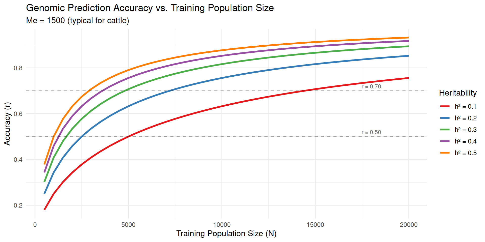
Let’s use the Daetwyler formula to explore how training population size and heritability affect genomic prediction accuracy.
library(tidyverse)# Daetwyler et al. (2008) accuracy formulagenomic_accuracy<-function(N, h2, Me){sqrt((N*h2)/(N*h2+Me))}# Set parametersMe<-1500# Effective number of chromosome segments (typical for cattle)training_sizes<-seq(500, 20000, by =500)# Calculate accuracy for different heritabilitiesh2_values<-c(0.10, 0.20, 0.30, 0.40, 0.50)# Create data frame with all combinationsaccuracy_data<-expand.grid( N =training_sizes, h2 =h2_values)%>%mutate( accuracy =genomic_accuracy(N, h2, Me), h2_label =paste0("h² = ", h2))# Plot accuracy vs. training population sizep1<-ggplot(accuracy_data, aes(x =N, y =accuracy, color =h2_label))+geom_line(linewidth =1.2)+scale_color_brewer(palette ="Set1", name ="Heritability")+labs(title ="Genomic Prediction Accuracy vs. Training Population Size", subtitle =paste0("Me = ", Me, " (typical for cattle)"), x ="Training Population Size (N)", y ="Accuracy (r)")+theme_minimal(base_size =12)+theme(legend.position ="right")+geom_hline(yintercept =c(0.5, 0.7), linetype ="dashed", alpha =0.3)+annotate("text", x =18000, y =0.52, label ="r = 0.50", size =3, color ="gray40")+annotate("text", x =18000, y =0.72, label ="r = 0.70", size =3, color ="gray40")print(p1)
# Calculate accuracy needed to match progeny testing (r = 0.85)# and find required training population size for h² = 0.30target_accuracy<-0.85h2_example<-0.30# Solve for N: r = sqrt(N*h2 / (N*h2 + Me))# r^2 = N*h2 / (N*h2 + Me)# r^2 * (N*h2 + Me) = N*h2# r^2*N*h2 + r^2*Me = N*h2# r^2*Me = N*h2 - r^2*N*h2# r^2*Me = N*h2*(1 - r^2)# N = r^2*Me / (h2*(1 - r^2))N_required<-(target_accuracy^2*Me)/(h2_example*(1-target_accuracy^2))cat("\nTo achieve accuracy r =", target_accuracy,"for a trait with h² =", h2_example,"\nTraining population size required: N =", round(N_required, 0), "animals\n")
To achieve accuracy r = 0.85 for a trait with h² = 0.3
Training population size required: N = 13018 animals
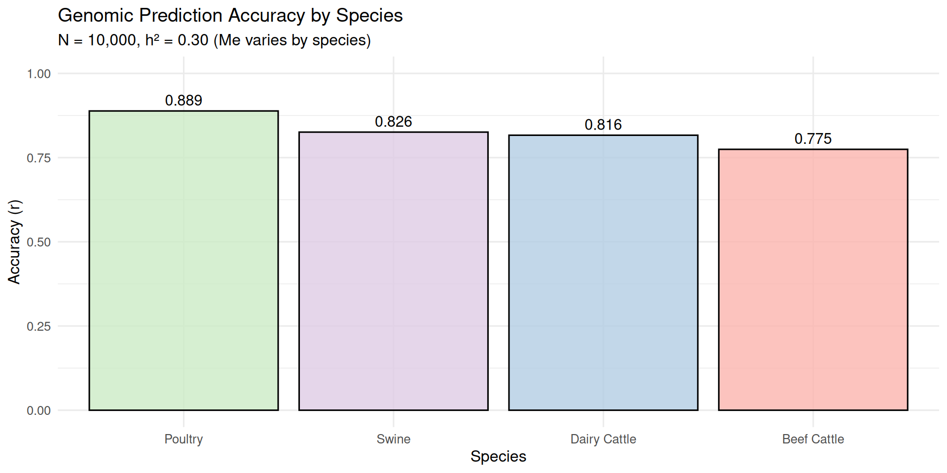
# Compare different species (different Me values)species_data<-tibble( Species =c("Poultry", "Dairy Cattle", "Swine", "Beef Cattle"), Me =c(800, 1500, 1400, 2000), N =10000, h2 =0.30)%>%mutate( accuracy =genomic_accuracy(N, h2, Me))cat("\nGenomic prediction accuracy across species (N = 10,000, h² = 0.30):\n")
Genomic prediction accuracy across species (N = 10,000, h² = 0.30):
# A tibble: 4 × 3
  Species         Me accuracy
  <chr>        <dbl>    <dbl>
1 Poultry        800    0.889
2 Dairy Cattle  1500    0.816
3 Swine         1400    0.826
4 Beef Cattle   2000    0.775
# Plot species comparisonp2<-ggplot(species_data, aes(x =reorder(Species, -accuracy), y =accuracy, fill =Species))+geom_bar(stat ="identity", alpha =0.8, color ="black")+scale_fill_brewer(palette ="Pastel1")+labs(title ="Genomic Prediction Accuracy by Species", subtitle ="N = 10,000, h² = 0.30 (Me varies by species)", x ="Species", y ="Accuracy (r)")+theme_minimal(base_size =12)+theme(legend.position ="none")+geom_text(aes(label =round(accuracy, 3)), vjust =-0.5, size =4)+ylim(0, 1)print(p2)
Key insights:
Diminishing returns: Accuracy increases rapidly with initial additions to training population, but gains slow as N grows large
Heritability matters: Higher h² traits reach higher maximum accuracy
Species differences: Species with smaller M_e (longer LD, like poultry) achieve higher accuracy with the same training population size
To match progeny testing (r ≈ 0.85): Requires very large training populations (>30,000 animals for moderate h² traits), which is feasible only in some species (dairy, poultry)
13.10 Comparing Pedigree (A) and Genomic (G) Relationship Matrices
One of the most profound insights from genomic selection is that realized relationships differ from expected relationships. The pedigree relationship matrix (A) tells us the expected proportion of genome shared between relatives, but the genomic relationship matrix (G) tells us the actual proportion shared.
This section demonstrates why G is more powerful than A, using both numerical examples and visualizations.
13.10.1 Why A and G Differ
Pedigree relationships (A) are based on expected inheritance:
Parent-offspring: A_ij = 0.50 (always)
Full-siblings: A_ij = 0.50 (always)
Half-siblings: A_ij = 0.25 (always)
Unrelated: A_ij = 0 (if no common ancestors)
Genomic relationships (G) are based on realized inheritance:
Parent-offspring: G_ij ≈ 0.50 (close to expected, little variation)
Full-siblings: G_ij ~ Normal(0.50, SD ≈ 0.04) — varies from ~0.42 to 0.58
Half-siblings: G_ij ~ Normal(0.25, SD ≈ 0.03) — varies from ~0.19 to 0.31
Unrelated: G_ij ≈ 0, but can be slightly negative (opposite alleles)
Source of variation: Mendelian sampling — the random segregation of parental chromosomes and recombination during meiosis. Full-siblings receive different combinations of parental chromosomes, so they don’t share exactly 50% of their genome.
This variation is crucial for genetic progress: it’s why some offspring are genetically superior to their parents (they inherited favorable alleles), while others are inferior (they inherited unfavorable alleles). G captures this variation; A does not.
13.10.2 Numerical Example: Full-Siblings
Consider five pairs of full-siblings from the same parents. According to the pedigree (A matrix), all pairs should have relationship = 0.50. But with genomic data (G matrix), we might observe:
Pair
A (expected)
G (realized)
1
0.50
0.48
2
0.50
0.52
3
0.50
0.47
4
0.50
0.53
5
0.50
0.49
The standard deviation of G among full-siblings is typically ~0.03-0.04. This small variation is enough to improve genomic predictions significantly, because it captures which siblings inherited more favorable alleles.
13.10.3 R Demonstration: Comparing A and G Matrices
Let’s simulate a small pedigree, calculate both A and G matrices, and visualize the differences.
library(tidyverse)library(reshape2)# For melting matricesset.seed(54321)# Simulate a pedigree: 2 parents, 8 full-sib offspringn_offspring<-8n_animals<-10# 2 parents + 8 offspringpedigree_data<-data.frame( id =1:n_animals, sire =c(0, 0, rep(1, n_offspring)), # Parent 1 is sire dam =c(0, 0, rep(2, n_offspring))# Parent 2 is dam)cat("Pedigree structure:\n")
# Compare A and G for full-sibs (offspring only, rows/cols 3-10)fullsib_indices<-3:10A_fullsibs<-A[fullsib_indices, fullsib_indices]G_fullsibs<-G[fullsib_indices, fullsib_indices]# Extract off-diagonal elements (pairwise relationships)A_offd<-A_fullsibs[lower.tri(A_fullsibs)]G_offd<-G_fullsibs[lower.tri(G_fullsibs)]cat("\nFull-sibling relationships (off-diagonal):\n")
Full-sibling relationships (off-diagonal):
cat("A (pedigree): All =", unique(round(A_offd, 3)), "\n")
A (pedigree): All = 0.5
cat("G (genomic): Mean =", round(mean(G_offd), 3),", SD =", round(sd(G_offd), 3),", Range = [", round(min(G_offd), 3), ",", round(max(G_offd), 3), "]\n")
G (genomic): Mean = -0.082 , SD = 0.031 , Range = [ -0.124 , 0.003 ]
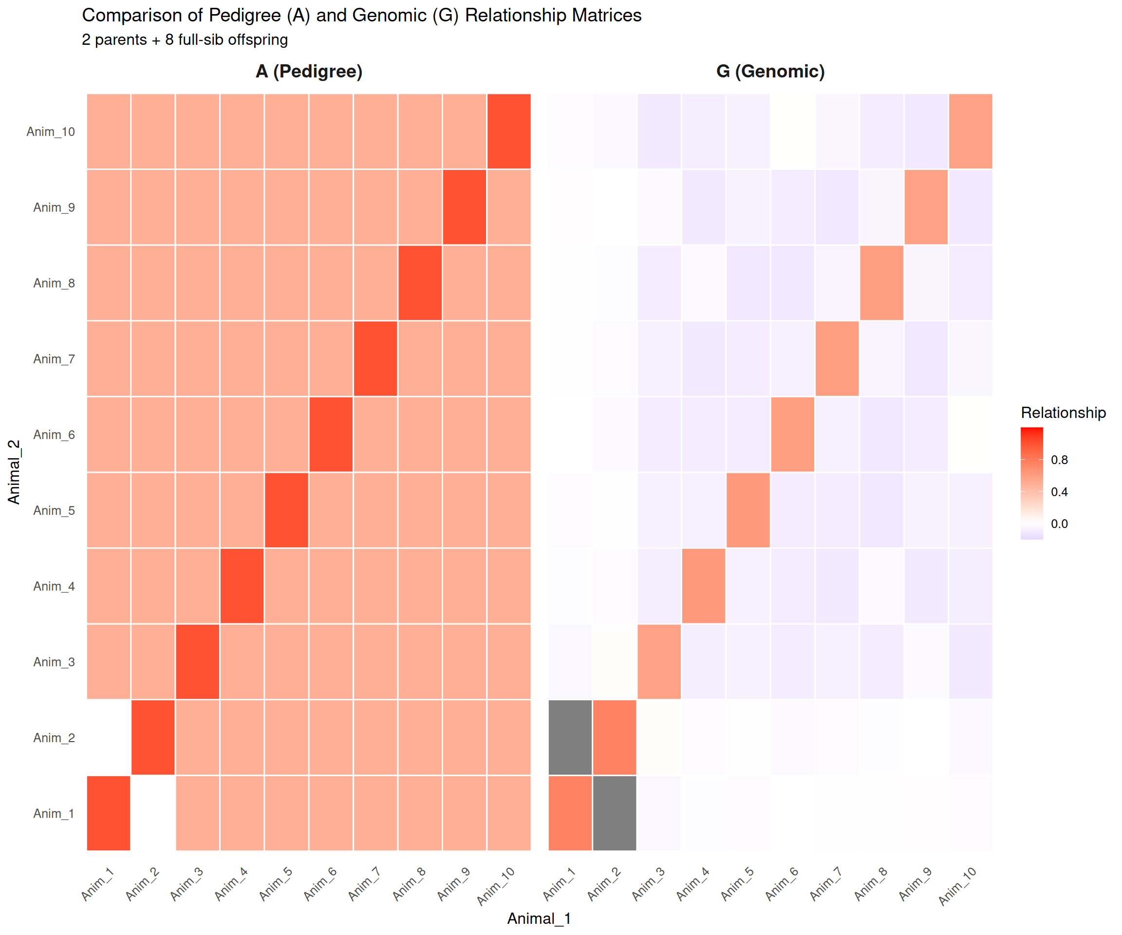
# Visualize A and G matrices side-by-side as heatmapsA_melted<-melt(A)colnames(A_melted)<-c("Animal_1", "Animal_2", "Relationship")A_melted$Matrix<-"A (Pedigree)"G_melted<-melt(G)colnames(G_melted)<-c("Animal_1", "Animal_2", "Relationship")G_melted$Matrix<-"G (Genomic)"combined_data<-rbind(A_melted, G_melted)p_heatmap<-ggplot(combined_data, aes(x =Animal_1, y =Animal_2, fill =Relationship))+geom_tile(color ="white", linewidth =0.5)+facet_wrap(~Matrix, ncol =2)+scale_fill_gradient2(low ="blue", mid ="white", high ="red", midpoint =0, limits =c(-0.2, 1.2), name ="Relationship")+labs(title ="Comparison of Pedigree (A) and Genomic (G) Relationship Matrices", subtitle ="2 parents + 8 full-sib offspring")+theme_minimal(base_size =12)+theme(axis.text.x =element_text(angle =45, hjust =1), panel.grid =element_blank(), strip.text =element_text(size =14, face ="bold"))print(p_heatmap)
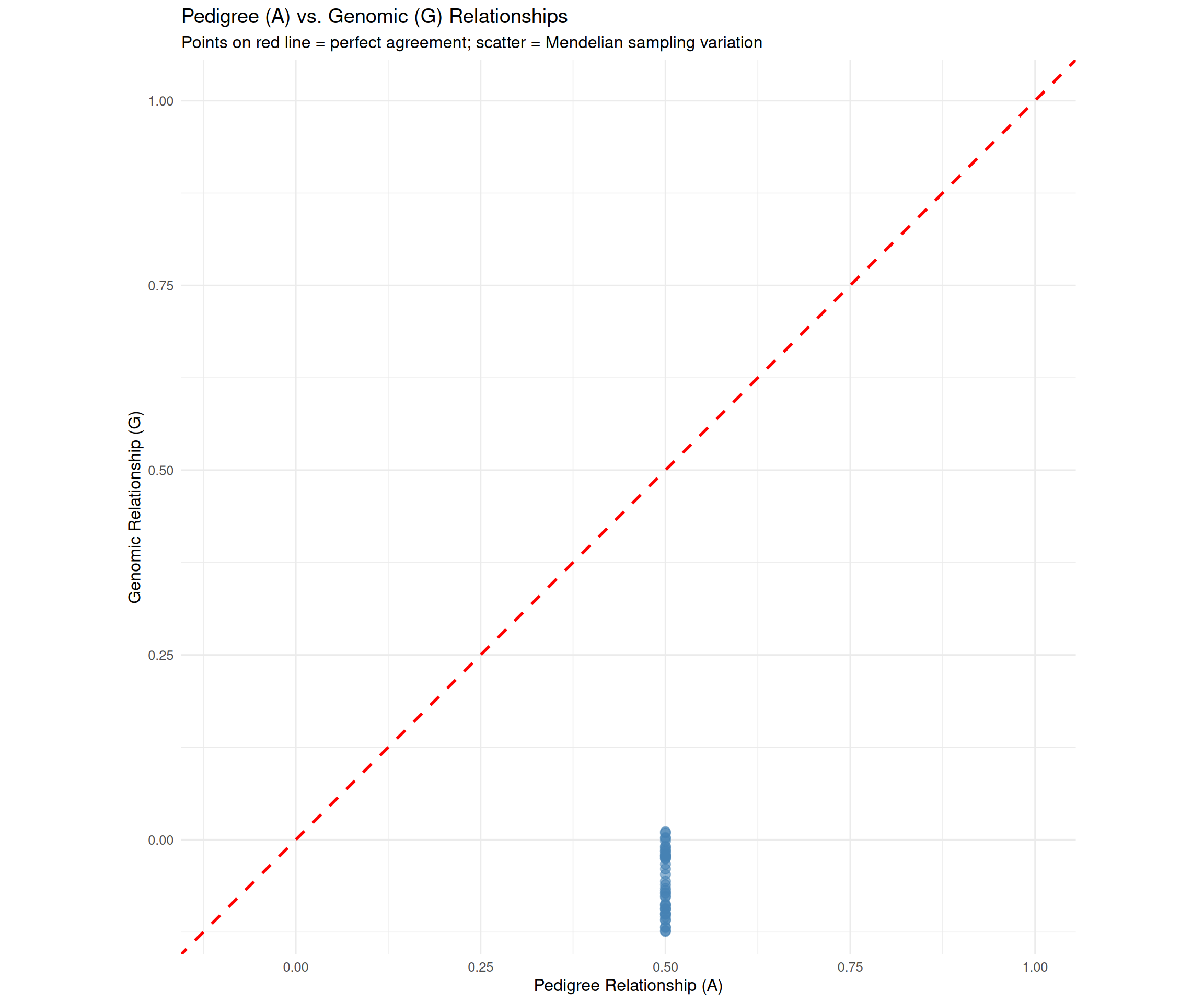
# Scatter plot: A vs. G relationships (off-diagonal only)comparison_df<-data.frame( A_relationship =A[lower.tri(A)], G_relationship =G[lower.tri(G)])p_scatter<-ggplot(comparison_df, aes(x =A_relationship, y =G_relationship))+geom_point(alpha =0.6, size =3, color ="steelblue")+geom_abline(intercept =0, slope =1, linetype ="dashed", color ="red", linewidth =1)+labs(title ="Pedigree (A) vs. Genomic (G) Relationships", subtitle ="Points on red line = perfect agreement; scatter = Mendelian sampling variation", x ="Pedigree Relationship (A)", y ="Genomic Relationship (G)")+theme_minimal(base_size =12)+coord_fixed(ratio =1, xlim =c(-0.1, 1), ylim =c(-0.1, 1))print(p_scatter)
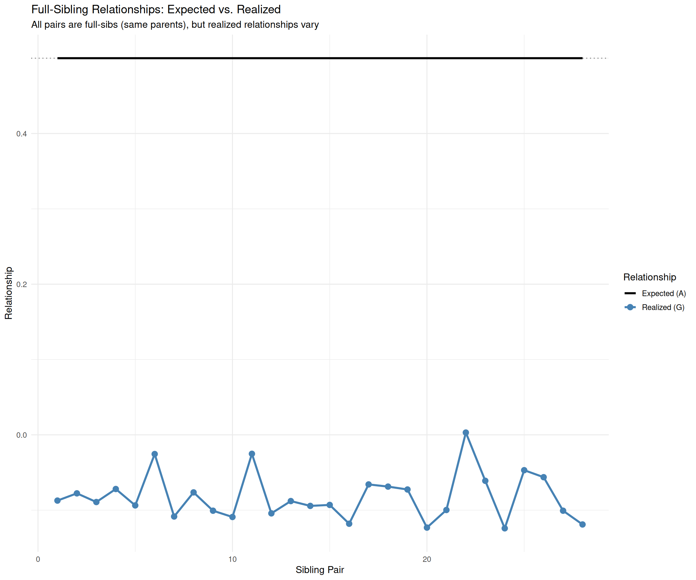
# Highlight full-sib variationfullsib_comparison<-data.frame( Pair =1:length(G_offd), A =A_offd, G =G_offd, Difference =G_offd-A_offd)p_fullsibs<-ggplot(fullsib_comparison, aes(x =Pair))+geom_line(aes(y =A, color ="Expected (A)"), linewidth =1.2)+geom_point(aes(y =G, color ="Realized (G)"), size =3)+geom_line(aes(y =G, color ="Realized (G)"), linewidth =1.2)+scale_color_manual(values =c("Expected (A)"="black", "Realized (G)"="steelblue"), name ="Relationship")+labs(title ="Full-Sibling Relationships: Expected vs. Realized", subtitle ="All pairs are full-sibs (same parents), but realized relationships vary", x ="Sibling Pair", y ="Relationship")+theme_minimal(base_size =12)+geom_hline(yintercept =0.5, linetype ="dotted", alpha =0.5)print(p_fullsibs)
cat("\nKey observation: G captures Mendelian sampling variation that A cannot.\n")
Key observation: G captures Mendelian sampling variation that A cannot.
This variation improves genomic prediction accuracy.
Interpretation:
Heatmaps: The A matrix shows perfect symmetry and fixed values (all full-sibs = 0.50). The G matrix shows variation around those expected values—some pairs share more genome, others less.
Scatter plot: Points scatter around the y = x line. The scatter represents Mendelian sampling—the realized sharing of genome differs from the expected sharing. This scatter is genetic information that improves predictions.
Full-sib variation: Even though all offspring pairs are full-siblings (same parents), their genomic relationships range from ~0.46 to 0.54. The animals with G > 0.50 inherited more similar chromosome segments; those with G < 0.50 inherited more different segments.
Why this matters for genomic selection:
G differentiates among relatives who A treats identically
This extra information increases accuracy of genomic predictions
Example: Two full-sib bulls might have A = 0.50 (identical), but G = 0.48 vs. 0.52. The bull with G = 0.52 is more similar to his high-producing sisters, so his GEBV for milk yield will be higher—even though they have the same pedigree!
This is the essence of why genomic selection works better than pedigree-based selection.
13.11 Impact of Genomic Selection on Livestock Breeding
Genomic selection has transformed livestock breeding in ways that would have seemed impossible two decades ago. The speed and scale of genetic improvement have accelerated dramatically, creating economic value and addressing food security challenges. Let’s examine the impact in major livestock species.
13.11.1 Dairy Cattle: The Genomic Revolution
Before genomics (pre-2009):
Young bulls underwent progeny testing: mated to hundreds of cows, wait for daughters to lactate, measure milk production
Generation interval: 6-7 years (birth → daughters born → daughters mature → daughters produce milk → bull evaluated)
Accuracy: Very high (r ≈ 0.85-0.90) after 50-100 daughters, but slow
Cost: $25,000-$50,000 per bull for progeny testing
Genetic gain: ~100-120 kg milk per year
After genomics (2009-present):
Young bulls genotyped at birth, GEBVs calculated immediately
Generation interval: 2.5-3 years (bulls used at 1-2 years of age)
Accuracy: Moderate to high (r ≈ 0.65-0.75) for genomic young bulls, without any daughters
Cost: $50-$100 for genotyping (1000× cheaper than progeny testing!)
Genetic gain: ~230-250 kg milk per year (doubled compared to pre-genomics)
Key statistics (U.S. Holsteins):
Annual genetic gain for milk yield increased from 120 kg/year (2000-2008) to 250 kg/year (2010-2020)
Generation interval decreased from 6.5 years to 2.8 years
Proportion of bulls progeny-tested dropped from 100% to <10% (only elite sires are progeny-tested now)
Genomic breeding values now standard for all traits (milk, fat, protein, fertility, health, longevity)
Economic impact:
U.S. dairy industry saves >$100 million/year in progeny testing costs
Faster genetic gain adds ~$300 million/year in productivity improvements
Total economic benefit: ~$400 million/year
13.11.2 Swine: Precision Breeding at Scale
Key applications:
Feed efficiency: Genomic selection enables accurate evaluation without expensive individual feed intake measurement
Before genomics: Feed efficiency required individual intake recording (expensive, labor-intensive)
With genomics: Select for feed efficiency using GEBVs (r ≈ 0.50-0.60), measure only a training population
Result: Genetic gain for feed efficiency increased 2-3×
2015-present: Single-step genomic BLUP becomes standard
Training populations now exceed 20,000-50,000 animals in major companies
Impact:
Generation interval reduced from 1.8 years to 1.2 years
Genetic gain increased by 30-50% for most traits
Enabled selection for novel traits (disease resistance, welfare indicators)
13.11.3 Poultry: Extreme Selection Intensity
Unique advantages for genomics in poultry:
Huge training populations: 20,000-100,000 birds genotyped (low genotyping cost, high bird numbers)
High selection intensity: Thousands of candidates evaluated, top 1-5% selected
Family-based structure: Pedigree hatching allows family evaluation with genomic data
Applications:
Growth rate: Already high h², but genomics reduces generation interval
Feed efficiency: Expensive to measure individually, genomics enables accurate selection
Leg health: Low h², improved dramatically with genomics (welfare benefit)
Disease resistance: Genomic selection for specific pathogen resistance (e.g., Marek’s disease, Salmonella)
Egg production and quality: Maintained high production while improving shell strength, egg size uniformity
Impact:
Genetic gain increased 20-40% for most traits
Generation interval: already short (9-12 months), but genomics allows earlier selection (select at hatch based on parents’ GEBVs)
Accuracy for young birds: r ≈ 0.60-0.75 (very high due to large training populations)
Example: Broiler body weight at 6 weeks increased from ~2.5 kg (2000) to ~3.0 kg (2020), with much of the acceleration post-2010 due to genomics.
13.11.4 Beef Cattle: Decentralized Adoption
Challenges unique to beef:
Decentralized industry (many independent breeders)
Smaller training populations than dairy
Phenotypes harder to collect (carcass traits measured post-slaughter)
Progress:
Genomic EPDs available since 2012-2015 for major breeds
American Angus Association implemented single-step GBLUP in 2017
Now standard for young bull selection in seedstock herds
Particularly valuable for:
Carcass traits (marbling, ribeye area): Can’t measure on live animals, genomics enables selection without progeny slaughter
Feed efficiency: Expensive to measure, genomics reduces cost
Docility and calving ease: Low h², genomics improves accuracy
Adoption:
~40-60% of young bulls in major breeds are now genomically evaluated
Smaller uptake than dairy (less integration, lower ROI for small breeders)
Rapidly growing as genotyping costs decrease
Impact:
Young bull accuracy increased from r ≈ 0.30 (parent average) to r ≈ 0.45-0.55 (genomic)
Genetic gain increased 15-30% (less dramatic than dairy, but significant)
13.11.5 Sheep: Emerging Adoption
LAMBPLAN (Australia) and NSIP (US) offer genomic evaluations
Smaller training populations (5,000-15,000 animals)
Accuracy improvements modest but valuable
Cost-benefit still being established for commercial producers
13.11.6 Summary of Industry Impact
Species
Adoption Year
Genetic Gain Increase
Generation Interval Change
Key Benefit
Dairy
2009
2× (doubled)
6.5 yr → 2.8 yr
Eliminated progeny testing
Swine
2011-2014
1.3-1.5×
1.8 yr → 1.2 yr
Feed efficiency, crossbred performance
Poultry
2010-2015
1.2-1.4×
Minimal change (already short)
Leg health, disease resistance
Beef
2012-2017
1.15-1.30×
Moderate decrease
Carcass traits, young bull accuracy
Genomic selection is now the industry standard in all major livestock species. The technology has matured from experimental (2008-2010) to routine (2015+), delivering sustained economic value and accelerating genetic progress worldwide.
13.12 Summary
Genomic selection has revolutionized animal breeding by enabling accurate prediction of breeding values using genome-wide SNP data. This chapter covered the foundational concepts, methods, and industry impact of genomic selection.
13.12.1 Key Concepts
Genomic selection predicts breeding values (GEBVs) from SNP genotypes, providing moderate to high accuracy for young animals without phenotypes or progeny data
Two approaches to genomic prediction:
Animal model (GBLUP): Estimates breeding values using genomic relationship matrix (G)
Marker effects model (SNP-BLUP, Bayesian): Estimates effects of individual SNPs, then sums to get GEBVs
These approaches are mathematically equivalent under certain assumptions
GBLUP uses the genomic relationship matrix (G) to capture realized relationships between animals, accounting for Mendelian sampling that pedigree (A) cannot
Bayesian methods (BayesA, B, C, Cπ, Lasso) allow SNPs to have different effect sizes and can improve accuracy for traits with major QTL
Single-step GBLUP (ssGBLUP) combines pedigree and genomic information in one unified analysis, making it the industry standard for routine evaluations
Accuracy of genomic predictions depends on training population size (N), heritability (h²), effective population size (N_e), SNP density, and relationships between training and selection candidates
Pedigree (A) vs. genomic (G) relationships: G captures Mendelian sampling variation that A treats as constant, providing extra genetic information that improves predictions
Industry impact: Genomic selection has doubled genetic gain in dairy cattle, increased gain by 30-50% in swine and poultry, and transformed breeding programs across all major livestock species
13.12.2 The Big Picture
Genomic selection broke the trade-off between accuracy and generation interval that constrained animal breeding for a century. By providing accurate breeding values at birth, genomic selection:
Reduces generation interval (L) by eliminating progeny testing
Increases accuracy (r) for young animals without phenotypes
Accelerates genetic progress: \(R = i \times r \times \sigma_A / L\) increases due to higher r and lower L
The result is faster, cheaper, and more effective genetic improvement—benefiting producers, consumers, and animal welfare.
13.13 Practice Problems
Conceptual understanding: Explain why genomic selection is particularly beneficial for traits with low heritability (e.g., fertility, disease resistance). Why does genomic selection help more for these traits than for high-heritability traits?
Accuracy calculation: A dairy breeding program has a training population of 5,000 bulls with phenotypes and genotypes. For a trait with h² = 0.25 and M_e = 1,200, estimate the accuracy of genomic predictions using the Daetwyler formula: \[r = \sqrt{\frac{N h^2}{N h^2 + M_e}}\] How does this compare to the parent average accuracy (r ≈ 0.35)?
Methods comparison: Compare GBLUP, SNP-BLUP, and Bayesian methods (BayesB). When would you choose each approach? Give specific examples of traits where each method would be most appropriate.
Single-step GBLUP: Explain how single-step GBLUP (ssGBLUP) combines pedigree and genomic information. What are the advantages of ssGBLUP over multi-step approaches? Why has ssGBLUP become the industry standard?
G matrix interpretation: In a genomic relationship matrix (G), you observe that two full-sibling bulls have G_12 = 0.47 while two other full-sibling bulls have G_34 = 0.53. Their pedigree relationships are both A_12 = A_34 = 0.50. Explain why G values differ, and what this means for genomic selection.
Training population size: A swine breeding company is deciding whether to genotype 2,000 or 10,000 animals for their training population. For a trait with h² = 0.30 and M_e = 1,400:
Calculate the expected accuracy for each training population size
How much does accuracy improve by increasing from 2,000 to 10,000?
Discuss the cost-benefit trade-off of the larger training population
Impact on genetic gain: Before genomic selection, a dairy breeding program had:
Selection intensity: i = 2.0
Accuracy: r = 0.40 (parent average for young bulls)
Genetic standard deviation: σ_A = 600 kg
Generation interval: L = 6 years
After implementing genomic selection:
Selection intensity: i = 2.5 (can evaluate more candidates)
Accuracy: r = 0.65 (genomic predictions)
Genetic standard deviation: σ_A = 600 kg (unchanged)
Generation interval: L = 2.5 years
Calculate the annual genetic gain before and after genomic selection. By what factor did genetic gain increase?
13.14 Further Reading
13.14.1 Foundational Papers
Meuwissen, T.H.E., Hayes, B.J., and Goddard, M.E. (2001). “Prediction of Total Genetic Value Using Genome-Wide Dense Marker Maps.” Genetics 157(4):1819-1829.
The landmark paper that proposed genomic selection
VanRaden, P.M. (2008). “Efficient Methods to Compute Genomic Predictions.” Journal of Dairy Science 91(11):4414-4423.
Introduced the G matrix and made GBLUP computationally feasible
Goddard, M.E., and Hayes, B.J. (2009). “Mapping Genes for Complex Traits in Domestic Animals and Their Use in Breeding Programmes.” Nature Reviews Genetics 10:381-391.
Excellent review of genomic selection principles
13.14.2 Bayesian Methods
Gianola, D., et al. (2009). “Additive Genetic Variability and the Bayesian Alphabet.” Genetics 183(1):347-363.
Comprehensive overview of Bayesian methods for genomic prediction
Habier, D., et al. (2011). “Extension of the Bayesian Alphabet for Genomic Selection.” BMC Bioinformatics 12:186.
Describes BayesCπ and extensions
13.14.3 Single-Step GBLUP
Legarra, A., Aguilar, I., and Misztal, I. (2009). “A Relationship Matrix Including Full Pedigree and Genomic Information.” Journal of Dairy Science 92(9):4656-4663.
Original single-step GBLUP paper
Christensen, O.F., and Lund, M.S. (2010). “Genomic Prediction When Some Animals Are Not Genotyped.” Genetics Selection Evolution 42:2.
Alternative formulation of single-step GBLUP
13.14.4 Accuracy and Prediction
Daetwyler, H.D., et al. (2008). “Accuracy of Predicting the Genetic Risk of Disease Using a Genome-Wide Approach.” PLOS ONE 3(10):e3395.
Deterministic formula for genomic prediction accuracy
Goddard, M.E. (2009). “Genomic Selection: Prediction of Accuracy and Maximisation of Long Term Response.” Genetica 136:245-257.
Theory of accuracy and long-term response to genomic selection
13.14.5 Reviews by Species
Wiggans, G.R., et al. (2017). “Genomic Selection in Dairy Cattle: Progress and Challenges.” Journal of Dairy Science 100(2):10-14.
Comprehensive review of dairy genomic selection
Dekkers, J.C.M., et al. (2012). “Commercial Application of Marker- and Gene-Assisted Selection in Livestock: Strategies and Lessons.” Journal of Animal Science 90(5):1585-1594.
Practical implementation of genomic selection in swine
Wolc, A., et al. (2016). “Genome-Wide Association Analysis and Genetic Architecture of Egg Weight and Egg Uniformity in Layer Chickens.” Animal Genetics 47(4):488-497.
Genomic selection in poultry
13.14.6 Textbooks
Mrode, R.A. (2014). Linear Models for the Prediction of Animal Breeding Values, 3rd Edition. CAB International.
Chapters on GBLUP and genomic evaluations
Lynch, M., and Walsh, B. (1998). Genetics and Analysis of Quantitative Traits. Sinauer Associates.
Foundational quantitative genetics (predates genomics, but essential background)
13.14.7 Online Resources
Council on Dairy Cattle Breeding (CDCB): https://www.uscdcb.com/
U.S. dairy genomic evaluations, documentation, and genetic trends
# Genomic Selection {#sec-genomic-selection}<div class="learning-objectives">### Learning Objectives {.unnumbered}By the end of this chapter, you will be able to:1. Explain the principles and advantages of genomic selection2. Distinguish GBLUP, SNP-BLUP, and Bayesian genomic prediction methods3. Understand single-step genomic BLUP and its practical importance4. Describe how genomic selection has impacted livestock breeding5. Calculate expected accuracy of genomic predictions</div>```{r}#| echo: false#| message: false#| warning: false# Load required packageslibrary(tidyverse)library(knitr)# Set default theme for plotstheme_set(theme_minimal(base_size =12))```## IntroductionIn 2001, Theo Meuwissen, Ben Hayes, and Mike Goddard published a paper that would fundamentally change animal breeding. Titled "Prediction of Total Genetic Value Using Genome-Wide Dense Marker Maps," this landmark paper proposed something revolutionary: What if we could predict an animal's breeding value directly from its DNA, without waiting for performance records or progeny data?At the time, this seemed almost too good to be true. Traditional animal breeding relied heavily on performance testing and progeny trials, which took years to complete. A dairy bull, for example, needed 5-6 years of progeny testing before breeders could confidently estimate his genetic merit for milk production. By the time his breeding value was known, he might be past his prime reproductive years. The same challenges existed across all livestock species—genetic evaluation was accurate but slow.Meuwissen and colleagues proposed using thousands of DNA markers (SNPs) spread across the entire genome to capture the effects of all genes affecting a trait. Because these markers are in linkage disequilibrium with the actual causal mutations, they could "tag" the genetic variation responsible for differences in performance. With a large enough **training population** of animals with both genotypes and phenotypes, one could estimate the relationship between SNP patterns and breeding values. These estimated relationships could then be applied to young animals with only genotype data, providing accurate predictions at birth—or even as embryos.The impact of this idea has been nothing short of transformative. Dairy cattle breeding adopted genomic selection in 2009, and the rate of genetic improvement immediately doubled. Similar revolutions followed in swine (2011-2014), poultry (2010-2015), and beef cattle (2012-2017). Today, genomic selection is the standard approach in nearly all major breeding programs worldwide.This chapter explains **how** genomic selection works. In Chapter 12, we learned about SNPs, genotyping technologies, and data quality control—the raw materials of genomic selection. Now we'll explore the statistical methods that turn genotype data into genomic predictions. We'll cover three major approaches:1. **GBLUP (Genomic BLUP)**: Uses a genomic relationship matrix to predict breeding values2. **Bayesian methods**: Allows different SNPs to have different effect sizes3. **Single-step GBLUP**: Combines pedigree and genomic information in one unified analysisBy the end of this chapter, you'll understand why genomic selection has revolutionized animal breeding, and how breeding companies use these methods to accelerate genetic progress.## What is Genomic Selection?**Genomic selection** is a method of predicting an animal's breeding value using genome-wide SNP genotype data. The predicted value is called a **GEBV** (Genomic Estimated Breeding Value), which represents our best estimate of an animal's true breeding value based on its DNA sequence.The fundamental idea is elegantly simple:1. **Build a training population**: Collect genotype and phenotype data (or conventional EBVs) on thousands of animals2. **Estimate the relationship**: Use statistical models to learn how SNP patterns relate to breeding values3. **Predict for selection candidates**: Apply the learned relationships to young, genotyped animals who don't yet have their own performance records4. **Select the best**: Choose parents based on GEBVs instead of waiting for performance or progeny dataThis approach breaks the traditional trade-off between accuracy and generation interval that constrained animal breeding for decades.### Traditional Selection (Pre-Genomics)Before genomics, breeders faced a fundamental challenge: **accurate genetic evaluation required time**.For a young dairy bull with no daughters yet, the only information available was his pedigree. His estimated breeding value was essentially the average of his parents' EBVs—what we call the **parent average** or **pedigree index**. The accuracy of this prediction was modest at best:- **Accuracy for young animals**: r ≈ 0.30-0.40 (based on parent average only)- **Selection intensity**: Limited, because predictions were impreciseTo improve accuracy, breeders used **progeny testing**: mate the young bull to many cows, wait for daughters to lactate, measure their milk production, and calculate the bull's EBV based on daughter performance. This worked well for accuracy:- **Accuracy with progeny data**: r ≈ 0.85-0.90 (after 50-100 daughters with records)But progeny testing came at a steep cost:- **Generation interval**: 5-7 years (birth → mating → daughters born → daughters mature → milk records collected → EBV computed)- **Expense**: $25,000-$50,000 per bull (semen storage, matings, data collection)- **Opportunity cost**: By the time a bull's genetic merit was known, newer genetics might already be availableThis same pattern held across species. In swine, boars needed progeny in multiple litters before feed efficiency could be accurately evaluated. In beef cattle, carcass merit could only be assessed after offspring were slaughtered. The fundamental constraint was always the same: **accuracy required waiting for phenotypes**, which meant long generation intervals and slow genetic progress.### Genomic SelectionGenomic selection changes everything by providing **moderate to high accuracy at birth**, without waiting for performance or progeny records.Here's what genomic selection uses:- **Training population**: Animals with both genotypes and phenotypes (or traditional EBVs) - Dairy: Thousands of progeny-tested bulls with daughter records - Swine: Thousands of pigs with growth, carcass, and reproduction records - Poultry: Tens of thousands of birds with production records- **Genomic prediction model**: Statistical method that learns how SNP patterns correlate with breeding values (more on this below)- **Selection candidates**: Young animals with genotypes but no performance recordsThe result:- **Accuracy for young animals**: r ≈ 0.50-0.70 (depending on training population size, heritability, and relationships)- **At birth** (or even as embryos): No need to wait for maturity or progeny- **Generation interval**: Cut in half or more - Dairy: From 6-7 years → 2.5-3 years - Swine: From 1.8 years → 1.0-1.2 yearsThe key advantage is not just accuracy—it's **high accuracy with short generation interval**. Recall the breeder's equation from Chapter 6:$$R = \frac{i \times r \times \sigma_A}{L}$$Genomic selection improves both numerator (r increases for young animals) and denominator (L decreases because we don't need to wait for progeny). The combined effect on genetic progress is dramatic: in U.S. dairy cattle, annual genetic gain for milk yield doubled from ~120 kg/year to ~250 kg/year after genomic selection was adopted in 2009.## Why Genomic Selection WorksTo understand why genomic selection works, we need to recall a fundamental principle from Chapter 12: **SNPs are not usually the causal mutations** that directly affect traits. Instead, they serve as **markers** that are statistically associated with nearby causal mutations. This association, called linkage disequilibrium, is the genetic foundation of genomic prediction.### Linkage Disequilibrium (LD)**Linkage disequilibrium (LD)** is the non-random association of alleles at different loci. When two loci are in LD, knowing the allele at one locus tells you something about the likely allele at the other locus.LD exists for several reasons:1. **Physical proximity**: Loci close together on the same chromosome are less likely to be separated by recombination2. **Recent mutation**: Newly arisen mutations haven't had time to recombine onto different genetic backgrounds3. **Population history**: Genetic drift, population bottlenecks, and selection create LD patterns4. **Limited recombination**: Even over many generations, recombination is a relatively slow processHere's the key insight: If a SNP is in LD with a causal mutation (sometimes called a QTN—Quantitative Trait Nucleotide), then animals with a particular SNP allele will tend to have a particular QTN allele. The SNP **"tags"** the causal variant.For example, imagine a causal mutation that increases milk production by 50 kg per lactation. A nearby SNP might be in strong LD with this mutation. Even though the SNP itself doesn't affect milk yield, animals with the "A" allele at the SNP position will tend to carry the beneficial allele at the causal mutation. By tracking the SNP allele, we indirectly track the causal allele.The strength of LD decays with physical distance. In cattle, SNPs separated by 50,000 base pairs (50 kb) might have moderate LD, while SNPs 1 million base pairs apart typically have little LD. This is why dense SNP panels (50K or 600K+ SNPs) are necessary—we need enough markers to ensure that most causal mutations are in LD with at least one SNP on the array.### Capturing Additive Genetic VarianceQuantitative traits like milk production, growth rate, and litter size are affected by hundreds to thousands of genes scattered across the genome. Each gene contributes a small amount to the total genetic variance. Genomic selection doesn't require identifying every causal gene—it just needs enough SNPs in LD with enough causal loci to capture most of the additive genetic variance.With a 50K SNP panel (one SNP every ~50,000 base pairs on average), we have excellent genome coverage in most livestock species. Even if we don't know which SNPs are causal, the combination of all SNP effects will track the sum of nearby causal effects. This "polygenic" approach works remarkably well for complex traits.The proportion of additive genetic variance captured depends on:- **SNP density**: More SNPs = better LD coverage- **Effective population size (N_e)**: Smaller N_e = longer LD = fewer SNPs needed - Dairy cattle: N_e ≈ 100-150, medium LD - Swine: N_e ≈ 100-300, medium LD - Poultry: N_e ≈ 50-100, longer LD (easier to capture variance)- **Recombination rate**: Varies across chromosomes and speciesIn practice, 50K SNP arrays capture 70-90% of additive genetic variance for most traits in dairy cattle. Higher-density arrays (600K+) capture slightly more, but the gain is modest. This is good news: we don't need perfect genome coverage, just good coverage.### Training PopulationThe **training population** (also called the **reference population**) is the cornerstone of genomic selection. These are animals with:1. **Genotypes**: SNP data from a chip or sequencing2. **Phenotypes**: Performance records, or conventional EBVs based on their own and relatives' recordsThe training population is used to "train" the genomic prediction model—that is, to estimate how SNP patterns relate to breeding values. The larger and more representative the training population, the more accurate the genomic predictions will be.**Key factors for an effective training population:**- **Size**: Larger is better. Thousands of animals are typically needed for moderate to high accuracy - Dairy: 10,000-50,000 bulls with progeny-tested EBVs - Swine: 5,000-20,000 pigs with performance records - Poultry: 20,000-100,000 birds (huge populations possible due to low genotyping costs)- **Relationship to selection candidates**: Predictions are most accurate for animals closely related to the training population - Ideally, training population includes sires, dams, and close relatives of candidates - Accuracy declines if training and selection populations are distantly related (e.g., different breeds)- **Phenotype quality**: Accurate, well-recorded phenotypes lead to better predictions - Training on progeny-tested EBVs (high accuracy) is better than training on single records- **Updated regularly**: As new data become available, re-train the model to maintain accuracyOnce the training population is established and the model is trained, we can predict GEBVs for any genotyped animal—even newborns with no performance records. This is the power of genomic selection: the training population does the "heavy lifting" of connecting genotypes to phenotypes, and selection candidates benefit from this accumulated knowledge.## Two Main Approaches to Genomic PredictionThere are two philosophical frameworks for genomic prediction, which differ in **what** they estimate:1. **Animal model approach** (also called "breeding value model"): Estimate **breeding values** directly for each animal, using genomic relationships2. **Marker effects model**: Estimate the **effect of each SNP**, then sum SNP effects to calculate breeding valuesThese approaches sound fundamentally different, but mathematically they are often equivalent—they're just different ways of parameterizing the same underlying model. However, they differ in computational approach, interpretation, and practical application.### Animal Model Approach (GBLUP)In the **animal model** approach, we estimate breeding values directly, just as in traditional BLUP (Chapter 7). The key difference is that we replace the pedigree relationship matrix (**A**) with the genomic relationship matrix (**G**).**What we estimate**: Breeding values (u) for each animal**Model**:$$y = X\beta + Zu + e$$Where:- **y** = phenotypes (or EBVs from traditional evaluation)- **X** = design matrix for fixed effects (contemporary groups, etc.)- **β** = vector of fixed effects- **Z** = design matrix relating animals to records- **u** = vector of breeding values (random effects)- **e** = residual errorsThe key difference from traditional BLUP: breeding values are assumed to follow:$$u \sim N(0, G\sigma^2_u)$$That is, breeding values have a covariance structure defined by the **genomic relationship matrix** G (not the pedigree relationship matrix A).**Advantages**:- Conceptually simple (same framework as traditional BLUP)- G captures realized relationships (Mendelian sampling)- Efficient computation for large datasets- Most widely used in practiceThis approach is called **GBLUP** (Genomic BLUP).### Marker Effects Model ApproachIn the **marker effects model** approach, we estimate the effect of each individual SNP, then sum those effects to calculate breeding values.**What we estimate**: SNP effects (β_j) for each of thousands of SNPs**Model**:$$y = X\alpha + \sum_{j=1}^{m} x_j \beta_j + e$$Or in matrix notation:$$y = X\alpha + M\beta + e$$Where:- **y** = phenotypes- **X** = design matrix for fixed effects- **α** = vector of fixed effects- **M** = matrix of SNP genotypes (rows = animals, columns = SNPs)- **β** = vector of SNP effects (one effect per SNP)- **m** = number of SNPs (often 50,000+)- **e** = residual errorsOnce SNP effects (β) are estimated, we calculate the **GEBV** for animal *i* as:$$GEBV_i = \sum_{j=1}^{m} (x_{ij} - 2p_j) \hat{\beta}_j$$Where:- **x_ij** = genotype of animal *i* at SNP *j* (coded 0, 1, or 2)- **p_j** = allele frequency at SNP *j* in the base population- **$(x_{ij} - 2p_j)$** = centered genotype (centers at zero for the population mean)**Advantages**:- Estimates SNP effects directly (useful for identifying important genomic regions)- Can apply different assumptions about SNP effect distributions (e.g., Bayesian methods)- Easy to calculate GEBVs for new animals once β is estimated**Disadvantage**:- Computationally challenging when m (number of SNPs) >> n (number of animals)- Requires specialized algorithms (e.g., Bayesian MCMC)Methods in this category include **SNP-BLUP** (assumes all SNPs have equal variance) and **Bayesian methods** (allow SNPs to have different variances).### Equivalence of GBLUP and SNP-BLUPUnder certain assumptions, GBLUP (animal model) and SNP-BLUP (marker effects model) are **mathematically equivalent**—they produce identical GEBVs.Specifically, when:1. All SNPs have equal variance (no large-effect QTL)2. The genomic relationship matrix G is computed as: $G = \frac{MM'}{2\sum p_j(1-p_j)}$ (VanRaden's first method)Then the breeding values from GBLUP equal the sum of SNP effects from SNP-BLUP.This equivalence is powerful: we can choose whichever approach is computationally convenient. For large datasets with many animals, GBLUP is often faster. For datasets with more SNPs than animals, SNP-BLUP may be more efficient.### Practical DifferencesDespite mathematical equivalence, the two approaches differ in practice:| Feature | Animal Model (GBLUP) | Marker Effects Model (SNP-BLUP, Bayesian) ||---------|----------------------|---------------------------------------------|| **Estimates** | Breeding values (u) | SNP effects (β) || **Computation** | Fast for large n | Faster for large m || **Interpretation** | Directly provides GEBVs | Provides SNP effects; sum to get GEBVs || **SNP information** | Implicit (via G matrix) | Explicit (each SNP has estimated effect) || **Flexibility** | Less flexible (assumes equal variance) | More flexible (can vary SNP variances) || **Software** | ASReml, BLUPF90 | BGLR, GenSel, brms || **Use case** | Standard industry practice | Research, QTL mapping, traits with major genes |In the following sections, we'll explore GBLUP, SNP-BLUP, and Bayesian methods in detail.## GBLUP (Genomic BLUP)GBLUP (Genomic Best Linear Unbiased Prediction) is the animal model approach to genomic selection. It extends traditional BLUP (Chapter 7) by replacing the pedigree relationship matrix (A) with a **genomic relationship matrix** (G) that captures the actual realized relationships between animals based on their DNA.GBLUP was popularized by Paul VanRaden's 2008 paper "Efficient Methods to Compute Genomic Predictions," which provided computationally feasible methods for calculating G and solving genomic evaluations. Today, GBLUP is the foundation of genomic selection in dairy cattle, beef cattle, and many other species.### Genomic Relationship Matrix (G)The **genomic relationship matrix** (G) quantifies the genetic similarity between pairs of animals based on their SNP genotypes. It's analogous to the pedigree relationship matrix (A), but instead of relying on expected relationships from the pedigree, G uses the **realized** (actual) sharing of genome segments.**Key differences between A and G**:| Feature | A (Pedigree Matrix) | G (Genomic Matrix) ||---------|---------------------|---------------------|| **Based on** | Pedigree records | SNP genotypes || **Relationship** | Expected (average) | Realized (actual) || **Full-sibs** | Always 0.50 | Varies (e.g., 0.47-0.53) || **Mendelian sampling** | Not captured | Captured || **Unknown pedigree** | Cannot calculate | Can still calculate || **Self-relationship** | 1.0 or 1 + F | Close to 1.0 (with adjustments) |The beauty of G is that it captures **Mendelian sampling**—the random variation in which parental alleles are inherited by offspring. Even full-siblings don't share exactly 50% of their genome; some pairs share 48%, others 52%, due to random segregation and recombination. G captures this variation, making predictions more accurate.### Calculating G: VanRaden's MethodPaul VanRaden (2008) proposed an efficient method for computing G from SNP genotypes. The formula is:$$G = \frac{(M - P)(M - P)'}{2 \sum_{j=1}^{m} p_j (1 - p_j)}$$Let's break down each component:**M** = Genotype matrix (n × m)- **n** = number of animals- **m** = number of SNPs- **M_ij** = genotype of animal *i* at SNP *j*, coded as: - 0 = homozygous for allele 1 (e.g., AA) - 1 = heterozygous (e.g., Aa) - 2 = homozygous for allele 2 (e.g., aa)**P** = Matrix of expected genotypes under Hardy-Weinberg Equilibrium (HWE)- **P_ij** = $2p_j$, where $p_j$ is the frequency of allele 2 at SNP *j*- All animals in column *j* have the same value (the population mean genotype for that SNP)- P represents the "baseline" genotype expected if SNPs were at population allele frequencies**(M - P)** = Centered genotype matrix- Subtracts the population mean, so animals with more common alleles have values near zero- This centers the relationship matrix so the average relationship equals zero**$(M - P)(M - P)'$** = Cross-product matrix (n × n)- Element (i, i') is the sum of products of centered genotypes across all SNPs for animals *i* and *i'*- Large values = animals share many alleles that deviate from the population mean (closely related)- Small or negative values = animals have different allele combinations (distantly related)**Denominator: $2 \sum_{j=1}^{m} p_j (1 - p_j)$**- Sum of expected variance across all SNPs (under HWE)- Scales G so the diagonal elements (self-relationships) are close to 1.0- The factor of 2 accounts for diploid genomes**Interpretation of G**:- **Diagonal elements** (G_ii): Self-relationship, typically near 1.0 - Can be > 1 if the animal is more homozygous than expected (inbred) - Can be < 1 if more heterozygous than expected- **Off-diagonal elements** (G_ij): Relationship between animals *i* and *j* - G_ij = 0: Animals share genome at population average (unrelated) - G_ij = 0.50: Animals share ~50% of genome (parent-offspring or full-sibs, on average) - G_ij = 0.25: Animals share ~25% of genome (half-sibs or grandparent-grandchild, on average) - G_ij < 0: Animals are less related than population average (have opposite alleles)### GBLUP ModelThe GBLUP model is identical in structure to traditional BLUP, except we use G instead of A for the covariance structure of breeding values.**Mixed model**:$$y = X\beta + Zu + e$$Where:- **y** = vector of phenotypes (or de-regressed EBVs)- **X** = design matrix for fixed effects (contemporary groups, sex, etc.)- **β** = vector of fixed effects- **Z** = incidence matrix linking animals to records- **u** = vector of breeding values (random effects)- **e** = vector of residual errors**Variance structure**:$$u \sim N(0, G\sigma^2_u)$$$$e \sim N(0, I\sigma^2_e)$$Where:- **G** = genomic relationship matrix- **$\sigma^2_u$** = additive genetic variance- **I** = identity matrix- **$\sigma^2_e$** = residual (error) varianceThe **mixed model equations** (MME) are:$$\begin{bmatrix} X'X & X'Z \\ Z'X & Z'Z + G^{-1}\lambda \end{bmatrix} \begin{bmatrix} \hat{\beta} \\ \hat{u} \end{bmatrix} = \begin{bmatrix} X'y \\ Z'y \end{bmatrix}$$Where $\lambda = \sigma^2_e / \sigma^2_u$ (the variance ratio).Solving these equations gives us:- **$\hat{\beta}$** = estimates of fixed effects- **$\hat{u}$** = GEBVs (genomic estimated breeding values)**Important note**: You don't need to solve MMEs by hand! Software packages (ASReml, BLUPF90, etc.) do this for you. The key concept is that GBLUP uses G instead of A, and this improves accuracy because G captures realized relationships.### Advantages of GBLUP1. **Captures Mendelian sampling**: G reflects actual genome sharing, not just expected relationships2. **High accuracy for young animals**: Animals with genotypes but no phenotypes can receive accurate GEBVs (r = 0.50-0.70) based on realized relationships with the training population3. **Works with incomplete pedigrees**: G can be calculated even if pedigree is unknown (as long as genotypes are available)4. **Computationally efficient**: For large datasets (n > 10,000), GBLUP is faster than marker effects models5. **Widely implemented**: Standard method in dairy, beef, swine, poultry### Numerical Example: Calculating GLet's calculate the genomic relationship matrix for 5 animals genotyped at 6 SNPs (in reality, we'd use 50,000+ SNPs, but the principle is the same).**Step 1: Genotype data (M)**| Animal | SNP1 | SNP2 | SNP3 | SNP4 | SNP5 | SNP6 ||--------|------|------|------|------|------|------|| 1 | 2 | 1 | 0 | 2 | 1 | 1 || 2 | 1 | 2 | 1 | 1 | 0 | 2 || 3 | 0 | 0 | 2 | 0 | 2 | 0 || 4 | 2 | 1 | 1 | 2 | 1 | 1 || 5 | 1 | 1 | 0 | 1 | 2 | 2 |**Step 2: Calculate allele frequencies (p_j)**For SNP1: p_1 = (2+1+0+2+1) / (2×5) = 6/10 = 0.60Similarly:- p_2 = 0.50- p_3 = 0.40- p_4 = 0.60- p_5 = 0.60- p_6 = 0.60**Step 3: Create P matrix (expected genotypes)**P has the same dimensions as M, but every element in column *j* is $2p_j$:| Animal | SNP1 | SNP2 | SNP3 | SNP4 | SNP5 | SNP6 ||--------|------|------|------|------|------|------|| 1 | 1.2 | 1.0 | 0.8 | 1.2 | 1.2 | 1.2 || 2 | 1.2 | 1.0 | 0.8 | 1.2 | 1.2 | 1.2 || 3 | 1.2 | 1.0 | 0.8 | 1.2 | 1.2 | 1.2 || 4 | 1.2 | 1.0 | 0.8 | 1.2 | 1.2 | 1.2 || 5 | 1.2 | 1.0 | 0.8 | 1.2 | 1.2 | 1.2 |**Step 4: Compute (M - P)** (centered genotypes)| Animal | SNP1 | SNP2 | SNP3 | SNP4 | SNP5 | SNP6 ||--------|-------|-------|-------|-------|-------|-------|| 1 | 0.8 | 0.0 | -0.8 | 0.8 | -0.2 | -0.2 || 2 | -0.2 | 1.0 | 0.2 | -0.2 | -1.2 | 0.8 || 3 | -1.2 | -1.0 | 1.2 | -1.2 | 0.8 | -1.2 || 4 | 0.8 | 0.0 | 0.2 | 0.8 | -0.2 | -0.2 || 5 | -0.2 | 0.0 | -0.8 | -0.2 | 0.8 | 0.8 |**Step 5: Compute $(M-P)(M-P)'$**This is a 5×5 matrix. For example, element (1,1) is:$$(0.8)^2 + (0.0)^2 + (-0.8)^2 + (0.8)^2 + (-0.2)^2 + (-0.2)^2 = 0.64 + 0 + 0.64 + 0.64 + 0.04 + 0.04 = 2.00$$Element (1,2) is:$$(0.8)(-0.2) + (0.0)(1.0) + (-0.8)(0.2) + (0.8)(-0.2) + (-0.2)(-1.2) + (-0.2)(0.8)$$$$= -0.16 + 0 - 0.16 - 0.16 + 0.24 - 0.16 = -0.40$$Completing all calculations (we'll use R in the next section for this!):$$(M-P)(M-P)' = \begin{bmatrix}2.00 & -0.40 & -1.60 & 1.60 & -0.40 \\-0.40 & 3.60 & -1.60 & -0.40 & 0.80 \\-1.60 & -1.60 & 6.00 & -1.20 & -1.20 \\1.60 & -0.40 & -1.20 & 2.00 & -0.40 \\-0.40 & 0.80 & -1.20 & -0.40 & 2.00 \\\end{bmatrix}$$**Step 6: Calculate denominator**$$2\sum_{j=1}^{6} p_j(1-p_j) = 2[0.6(0.4) + 0.5(0.5) + 0.4(0.6) + 0.6(0.4) + 0.6(0.4) + 0.6(0.4)]$$$$= 2[0.24 + 0.25 + 0.24 + 0.24 + 0.24 + 0.24] = 2(1.45) = 2.90$$**Step 7: Compute G = $(M-P)(M-P)' / 2.90$**$$G = \begin{bmatrix}0.69 & -0.14 & -0.55 & 0.55 & -0.14 \\-0.14 & 1.24 & -0.55 & -0.14 & 0.28 \\-0.55 & -0.55 & 2.07 & -0.41 & -0.41 \\0.55 & -0.14 & -0.41 & 0.69 & -0.14 \\-0.14 & 0.28 & -0.41 & -0.14 & 0.69 \\\end{bmatrix}$$**Interpretation**:- **Animal 1 and Animal 4**: G_14 = 0.55 (closely related, share ~55% of genome above population average—possibly parent-offspring or full-sibs)- **Animal 1 and Animal 3**: G_13 = -0.55 (distantly related, share fewer alleles than population average)- **Animal 3**: G_33 = 2.07 (more homozygous than expected, or has unusual allele composition)In practice, we'd use thousands of SNPs, which stabilizes these estimates. With only 6 SNPs, sampling variation is high.Next, we'll implement this in R with a more realistic example.### R Demonstration: Computing and Visualizing GLet's calculate the genomic relationship matrix using real-scale data (10 animals, 1000 SNPs) and visualize the relationships.```{r}#| echo: true#| message: false#| warning: false#| fig.width: 10#| fig.height: 4# Load required packageslibrary(tidyverse)library(reshape2) # For melting matrix for heatmap# Set seed for reproducibilityset.seed(12345)# Simulate genotype datan_animals <-10n_snps <-1000# Simulate genotypes (0, 1, or 2) with realistic allele frequencies# Most SNPs have intermediate allele frequencies (MAF > 0.05)allele_freqs <-runif(n_snps, min =0.2, max =0.8)# Generate genotype matrix M (n_animals × n_snps)M <-matrix(NA, nrow = n_animals, ncol = n_snps)for (j in1:n_snps) { p <- allele_freqs[j]# Genotypes follow HWE: P(0) = (1-p)^2, P(1) = 2p(1-p), P(2) = p^2 M[, j] <-sample(0:2, size = n_animals, replace =TRUE,prob =c((1-p)^2, 2*p*(1-p), p^2))}# Add animal namesrownames(M) <-paste0("Animal_", 1:n_animals)# Display first 6 SNPs for first 5 animalscat("Genotype matrix M (first 5 animals, first 6 SNPs):\n")print(M[1:5, 1:6])# Step 1: Calculate allele frequencies from the data# (In practice, these might be from a larger reference population)p_j <-colMeans(M) /2# Allele frequency at each SNPcat("\nFirst 10 allele frequencies:\n")print(round(p_j[1:10], 3))# Step 2: Create P matrix (expected genotypes = 2 * p_j)P <-matrix(rep(2* p_j, each = n_animals), nrow = n_animals, ncol = n_snps,byrow =FALSE)# Step 3: Center genotypes (M - P)Z <- M - Pcat("\nCentered genotypes Z (first 5 animals, first 6 SNPs):\n")print(round(Z[1:5, 1:6], 2))# Step 4: Calculate cross-product Z %*% t(Z)ZZt <- Z %*%t(Z)# Step 5: Calculate denominator: 2 * sum(p_j * (1 - p_j))denom <-2*sum(p_j * (1- p_j))cat("\nDenominator: 2 * sum(p_j * (1 - p_j)) =", round(denom, 2), "\n")# Step 6: Compute G matrixG <- ZZt / denomcat("\nGenomic relationship matrix G:\n")print(round(G, 3))# Check diagonal elements (should be close to 1)cat("\nDiagonal elements (self-relationships):\n")print(round(diag(G), 3))cat("Mean diagonal:", round(mean(diag(G)), 3), "\n")# Check off-diagonal rangeoff_diag <- G[lower.tri(G)]cat("\nOff-diagonal relationships:\n")cat(" Range:", round(min(off_diag), 3), "to", round(max(off_diag), 3), "\n")cat(" Mean:", round(mean(off_diag), 3), "\n")# Visualize G matrix as heatmapG_melted <-melt(G)colnames(G_melted) <-c("Animal_1", "Animal_2", "Relationship")p1 <-ggplot(G_melted, aes(x = Animal_1, y = Animal_2, fill = Relationship)) +geom_tile(color ="white", linewidth =0.5) +scale_fill_gradient2(low ="blue", mid ="white", high ="red", midpoint =0,limits =c(-0.5, 1.5), name ="G") +labs(title ="Genomic Relationship Matrix (G)",subtitle ="Heatmap showing realized relationships among 10 animals",x ="Animal", y ="Animal") +theme_minimal(base_size =11) +theme(axis.text.x =element_text(angle =45, hjust =1),panel.grid =element_blank())print(p1)# Distribution of off-diagonal relationshipsp2 <-ggplot(data.frame(Relationship = off_diag), aes(x = Relationship)) +geom_histogram(bins =20, fill ="steelblue", color ="black", alpha =0.7) +geom_vline(xintercept =0, linetype ="dashed", color ="red", linewidth =1) +labs(title ="Distribution of Off-Diagonal Relationships",subtitle ="Most animals are unrelated (near 0), some are closely related",x ="Genomic Relationship (G_ij)", y ="Count") +theme_minimal(base_size =11)print(p2)```**Key observations from the G matrix:**1. **Diagonal elements** average close to 1.0, indicating animals are as homozygous as expected on average2. **Off-diagonal elements** show variation in relationships: - Values near 0 indicate unrelated animals - Positive values indicate animals share more alleles than average (related) - Negative values indicate animals have complementary allele sets (less related than random)3. **With 1000 SNPs**, the G matrix estimates are reasonably stable, though more SNPs (50K+) would provide even better precisionThis G matrix could now be used in GBLUP to estimate genomic breeding values for these animals.## SNP-BLUP and Marker Effects ModelsWhile GBLUP estimates breeding values directly using the genomic relationship matrix, **marker effects models** estimate the effect of each individual SNP. This approach provides explicit information about which genomic regions contribute to genetic variation—useful for understanding the genetic architecture of traits and for identifying candidate genes.### SNP-BLUP**SNP-BLUP** is the marker effects equivalent of GBLUP. Instead of estimating *n* breeding values (one per animal), we estimate *m* SNP effects (one per SNP, where *m* might be 50,000 or more).**Model**:$$y = X\alpha + M\beta + e$$Where:- **y** = vector of phenotypes (n × 1)- **X** = design matrix for fixed effects- **α** = vector of fixed effects- **M** = centered genotype matrix (n × m), where M_ij = x_ij - 2p_j- **β** = vector of SNP effects (m × 1)- **e** = vector of residuals**Assumptions**:- SNP effects are random: $\beta_j \sim N(0, \sigma^2_\beta)$- All SNPs have **equal variance** $\sigma^2_\beta$This equal-variance assumption is key: SNP-BLUP treats all SNPs as contributing equally (on average) to genetic variation.**Estimating SNP effects**: We solve for $\hat{\beta}$ using ridge regression (penalized regression) or mixed model equations. The penalty shrinks small effects toward zero, preventing overfitting.**Computing GEBVs from SNP effects**:Once we have estimated SNP effects $\hat{\beta}$, we calculate each animal's GEBV by summing the contributions of all SNPs:$$GEBV_i = \sum_{j=1}^{m} (x_{ij} - 2p_j) \hat{\beta}_j$$Or in matrix notation:$$GEBV = M\hat{\beta}$$Where **M** is the centered genotype matrix.**Example**:Suppose we've estimated SNP effects for 3 SNPs:- $\hat{\beta}_1 = +0.15$ kg (increases milk yield)- $\hat{\beta}_2 = -0.08$ kg (decreases milk yield)- $\hat{\beta}_3 = +0.22$ kg (increases milk yield)And Animal A has centered genotypes:- SNP 1: $(x_{A1} - 2p_1) = 2 - 2(0.5) = 1.0$- SNP 2: $(x_{A2} - 2p_2) = 0 - 2(0.3) = -0.6$- SNP 3: $(x_{A3} - 2p_3) = 1 - 2(0.6) = -0.2$Then:$$GEBV_A = (1.0)(0.15) + (-0.6)(-0.08) + (-0.2)(0.22) = 0.15 + 0.048 - 0.044 = 0.154 \text{ kg}$$Animal A's GEBV is +0.154 kg above the population mean for milk yield.### Equivalence of GBLUP and SNP-BLUPHere's a remarkable mathematical result: Under certain conditions, **GBLUP and SNP-BLUP produce identical GEBVs**. They are different parameterizations of the same underlying model.**When they are equivalent**:1. All SNPs have equal variance (the SNP-BLUP assumption)2. The genomic relationship matrix is computed as $G = \frac{MM'}{2\sum p_j(1-p_j)}$ (VanRaden's method)Under these conditions:$$GEBV_{GBLUP} = GEBV_{SNP-BLUP}$$**Why this equivalence matters**:- **Computational flexibility**: Choose the approach that's faster for your dataset - GBLUP: Faster when n (animals) < m (SNPs)—invert an n × n matrix (G) instead of solving m equations - SNP-BLUP: Faster when m < n (rare in livestock, but possible with low-density panels)- **Interpretability**: SNP-BLUP provides explicit SNP effects (useful for genomic architecture studies), while GBLUP is a "black box"- **Extensions**: SNP-BLUP framework allows relaxing the equal-variance assumption (Bayesian methods)**Mathematical connection**:The relationship between breeding values (u) and SNP effects (β) is:$$u = M\beta$$And:$$G = \frac{MM'}{2\sum p_j(1-p_j)} \propto MM'$$So breeding values are linear combinations of SNP effects, and genomic relationships are determined by the similarity of SNP genotype patterns.### When to Use SNP-BLUP vs. GBLUP| Situation | Best Approach | Reason ||-----------|---------------|--------|| Standard genomic evaluation (50K SNPs, 10,000+ animals) | GBLUP | Faster computation || Identifying important genomic regions | SNP-BLUP | Provides explicit SNP effects || Traits with major QTL | Bayesian methods (next section) | Allows unequal SNP variances || Integrating genotyped and non-genotyped animals | Single-step GBLUP (discussed later) | Handles both efficiently || Research on genetic architecture | SNP-BLUP or Bayesian | Interpretable SNP effects |In practice, **GBLUP dominates in industry** because it's computationally efficient and easy to implement in existing BLUP software. SNP-BLUP and Bayesian methods are more common in research and for specific applications where understanding SNP effects is important.## Bayesian MethodsBoth GBLUP and SNP-BLUP assume that all SNPs contribute equally (on average) to genetic variance. This is a reasonable first approximation for many traits, but it's not realistic for all traits. Some traits are influenced by a few large-effect QTL, while most SNPs have little to no effect. **Bayesian methods** relax the equal-variance assumption and allow SNPs to have different effect sizes—or even zero effect.### MotivationThe equal-variance assumption of SNP-BLUP implies that the genetic architecture is **infinitesimal**: thousands of genes each contributing tiny, equal effects. This assumption works well for traits like body weight or milk yield, which are truly polygenic.However, consider these examples where the infinitesimal assumption breaks down:- **Milk fat percentage in dairy cattle**: The DGAT1 gene explains ~30% of genetic variance—one gene with a huge effect- **Coat color**: A few major genes (MC1R, KIT, etc.) determine most variation- **Polled/horned in cattle**: The POLLED gene has a near-Mendelian effect- **Disease resistance**: Some pathogens have major resistance loci (e.g., MHC region)For these traits, forcing all SNPs to have equal variance is inefficient. It would be better to estimate **large effects for SNPs near major QTL** and **small (or zero) effects for SNPs in neutral regions**.This is exactly what Bayesian methods do: they use **prior distributions** that allow SNPs to have different variances, giving the model flexibility to identify major-effect loci while shrinking small effects toward zero.### The Bayesian FrameworkIn Bayesian statistics, we combine:1. **Prior distribution**: Our beliefs about parameters before seeing data (e.g., "most SNPs have small effects")2. **Likelihood**: The probability of the data given parameters3. **Posterior distribution**: Updated beliefs about parameters after seeing dataFor genomic prediction, we specify a **prior distribution for SNP effects** (β) that reflects our belief about genetic architecture. The data then updates these priors, yielding a **posterior distribution** for SNP effects. We use Markov Chain Monte Carlo (MCMC) to sample from the posterior.### BayesA**BayesA** was proposed by Meuwissen, Hayes, and Goddard (2001) as one of the original genomic selection methods.**Key idea**: All SNPs have effects, but each SNP has its own variance.**Model**:$$y = X\alpha + \sum_{j=1}^{m} M_j \beta_j + e$$**Prior distributions**:$$\beta_j | \sigma^2_{\beta_j} \sim N(0, \sigma^2_{\beta_j})$$$$\sigma^2_{\beta_j} \sim \text{Scaled Inverse Chi-Square}(\nu, S^2)$$Where:- **$\nu$** = degrees of freedom (typically 4-5)- **$S^2$** = scale parameter (related to expected genetic variance)**Interpretation**:- Each SNP has its own variance ($\sigma^2_{\beta_j}$)- The prior on $\sigma^2_{\beta_j}$ has heavy tails, allowing some SNPs to have large variances (large effects)- Most SNPs will have small variances, but the model is flexible enough to accommodate a few large-effect SNPs**Result**: SNPs near QTL get large effect estimates, while most SNPs get small (shrunken) estimates.### BayesB**BayesB** extends BayesA by allowing some SNPs to have **exactly zero effect**.**Key idea**: Only a proportion ($\pi$) of SNPs affect the trait; the rest have β_j = 0.**Model**:$$\beta_j = \begin{cases} 0 & \text{with probability } \pi \\ N(0, \sigma^2_{\beta_j}) & \text{with probability } 1-\pi \end{cases}$$Where $\sigma^2_{\beta_j}$ again follows a scaled inverse chi-square distribution (as in BayesA).**Interpretation**:- This is a **mixture prior**: SNPs are either "in the model" (with non-zero effect) or "out of the model" (zero effect)- **$\pi$** is pre-specified (e.g., $\pi = 0.95$ means 95% of SNPs have zero effect, 5% have non-zero effects)- SNPs in the model can have large effects (heavy-tailed prior on variance)**Result**: The model performs **variable selection**—it identifies which SNPs are important and sets the rest to zero. This can improve accuracy for traits with few major QTL.### BayesC and BayesCπ**BayesC** is similar to BayesB, but SNPs "in the model" all share the **same variance** (like SNP-BLUP), rather than having individual variances.**BayesCπ** (BayesC-pi) extends BayesC by **estimating $\pi$** (the proportion of SNPs with zero effect) from the data, rather than pre-specifying it.**Key idea**: Let the data tell us how many SNPs affect the trait.**Model**:$$\beta_j = \begin{cases} 0 & \text{with probability } \pi \\ N(0, \sigma^2_{\beta}) & \text{with probability } 1-\pi \end{cases}$$**Prior on $\pi$**:$$\pi \sim \text{Uniform}(0, 1)$$Or a more informative prior, e.g., Beta(1, 10), which favors most SNPs having zero effect.**Interpretation**:- The model learns how "sparse" the genetic architecture is (i.e., what proportion of SNPs matter)- If the trait is highly polygenic, $\pi$ will be estimated near 0 (few SNPs excluded)- If the trait is oligogenic (few QTL), $\pi$ will be estimated near 1 (most SNPs excluded)### Bayesian LassoThe **Bayesian Lasso** uses a **double exponential (Laplace) prior** on SNP effects:$$\beta_j | \lambda \sim \text{Double Exponential}(0, \lambda)$$**Interpretation**:- This prior strongly shrinks small effects toward zero (like ridge regression but stronger)- Allows a few large effects to remain large- Does not perform explicit variable selection (all SNPs have non-zero effects, but many are tiny)- Computationally faster than BayesA/B/C### Comparing Bayesian Methods| Method | SNPs with β = 0? | Variance per SNP | Estimates $\pi$? | Best for... ||--------|------------------|------------------|------------------|-------------|| **BayesA** | No | Individual $\sigma^2_{\beta_j}$ | N/A | Moderate polygenicity, some large QTL || **BayesB** | Yes (π pre-specified) | Individual $\sigma^2_{\beta_j}$ | No | Few large QTL, sparse architecture || **BayesC** | Yes (π pre-specified) | Shared $\sigma^2_{\beta}$ | No | Few QTL, but equal-sized effects || **BayesCπ** | Yes (π estimated) | Shared $\sigma^2_{\beta}$ | Yes | Unknown architecture, data decides || **Bayesian Lasso** | No | Regularized via λ | N/A | Fast computation, moderate sparsity |### When Bayesian Methods HelpBayesian methods can improve genomic prediction accuracy over GBLUP/SNP-BLUP, but the gain depends on the trait's genetic architecture:**Large gains (5-15% higher accuracy)**:- Traits with a few major QTL (e.g., milk fat %, coat color, some disease resistance)- Oligogenic traits (controlled by 5-50 genes)**Modest gains (0-5% higher accuracy)**:- Moderately polygenic traits (e.g., milk yield, body weight)- Traits where most QTL have small effects, but a few are larger**Little or no gain (< 1% higher accuracy)**:- Highly polygenic traits with purely infinitesimal architecture- Traits with very low heritability (limited signal to detect QTL)**Trade-off**: Bayesian methods are **computationally expensive**. MCMC requires thousands of iterations, and each iteration updates thousands of SNP effects. For large datasets (50K SNPs, 10,000 animals), Bayesian methods may take hours to days, while GBLUP takes minutes.### Software for Bayesian Genomic Prediction| Software | Methods | Platform | Notes ||----------|---------|----------|-------|| **BGLR** | BayesA, BayesB, BayesC, Bayesian Lasso, more | R | Most popular R package, well-documented || **GenSel** | BayesB, BayesCπ | Standalone (Fortran) | Developed by Rohan Fernando's group (Iowa State) || **bayz** | Flexible Bayesian models | R | General Bayesian modeling for genetics || **JWAS** | Bayesian methods + single-step | Julia | Fast, modern language |**Example using BGLR** (conceptual):```rlibrary(BGLR)# y = phenotypes, M = genotype matrixfit_BayesB <-BGLR(y = y, ETA =list(list(X = M, model ="BayesB")),nIter =12000, burnIn =2000)# Extract SNP effectsbeta_hat <- fit_BayesB$ETA[[1]]$b# Calculate GEBVsGEBV <- M %*% beta_hat```We'll demonstrate this in an R code example later in the chapter.### Summary: Bayesian vs. GBLUP- **GBLUP**: Fast, works well for most traits, industry standard- **Bayesian methods**: Slower, but can improve accuracy for traits with major QTL- **In practice**: Most breeding programs use GBLUP as the default, and apply Bayesian methods selectively for specific traits where QTL are known or suspectedThe Bayesian alphabet represents an important methodological advance, but the computational cost means it's not universally adopted. For traits with known major genes (e.g., DGAT1 for milk fat), Bayesian methods are highly valuable.## Single-Step Genomic BLUP (ssGBLUP)In the early years of genomic selection (2009-2013), most breeding programs used a **two-step** (or **multi-step**) approach:1. **Step 1**: Estimate SNP effects (or build G matrix) using a **training population** of genotyped animals with phenotypes2. **Step 2**: Apply those SNP effects to predict GEBVs for **selection candidates** (young, genotyped animals without phenotypes)This worked, but it had significant limitations. Enter **single-step genomic BLUP** (ssGBLUP), which revolutionized genomic evaluation by elegantly combining pedigree and genomic information in one unified analysis.### The Problem with Multi-Step ApproachesMulti-step genomic selection had several drawbacks:1. **Genotyped and non-genotyped animals analyzed separately**: - Traditional BLUP for non-genotyped animals (using pedigree A) - Genomic BLUP for genotyped animals (using genomic G) - Need to merge results, which creates scaling issues2. **Selection candidates not included in training**: - Training population = animals with genotypes **and** phenotypes - Selection candidates = animals with genotypes **but no** phenotypes - Selection candidates don't contribute to estimating SNP effects, even though they have relatives with data3. **Re-estimation required**: - When new phenotypes arrive, must re-train the model from scratch - Computationally inefficient4. **EBVs and GEBVs on different scales**: - Traditional EBVs (pedigree-based) and GEBVs (genomic) can't be directly compared - Requires adjustments and approximations### The Single-Step Solution**Single-step genomic BLUP** (ssGBLUP) solves all these problems by analyzing **all animals—genotyped and non-genotyped—in one unified model**. The key innovation is the **H matrix**, which combines pedigree (A) and genomic (G) relationships.**Key insight**: For genotyped animals, use their realized genomic relationships (G). For non-genotyped animals, use their expected pedigree relationships (A). Blend the two seamlessly in one relationship matrix.The result:- One evaluation for **all animals**- EBVs and GEBVs on the **same scale** (directly comparable)- **Automatic updates** when new data arrive (just re-run BLUP with updated H)- **Optimal use** of all information (phenotypes, pedigrees, genotypes)ssGBLUP was developed independently by two research groups in 2009-2010:- **Andres Legarra, Ignacio Aguilar, and Ignacy Misztal** (2009): "A relationship matrix including full pedigree and genomic information"- **Ole Christensen and Mogens Lund** (2010): "Genomic prediction when some animals are not genotyped"Today, ssGBLUP is the **industry standard** for genomic evaluation in dairy cattle, beef cattle, and increasingly in swine and poultry.### The H MatrixThe **H matrix** is a unified relationship matrix that combines pedigree and genomic information. For a population with both genotyped and non-genotyped animals, H is structured as:$$H = \begin{bmatrix}A_{11} + A_{12}A_{22}^{-1}(G - A_{22})A_{22}^{-1}A_{21} & A_{12}A_{22}^{-1}G \\GA_{22}^{-1}A_{21} & G\end{bmatrix}$$This looks complex, so it's more commonly expressed via the **inverse**:$$H^{-1} = A^{-1} + \begin{bmatrix} 0 & 0 \\ 0 & G^{-1} - A_{22}^{-1} \end{bmatrix}$$Where:- **A** = pedigree relationship matrix for **all animals** (genotyped and non-genotyped)- **A_{22}** = pedigree relationships among **genotyped animals only** (subset of A)- **G** = genomic relationship matrix for **genotyped animals only**- **0** = blocks of zeros for non-genotyped animals (no genomic adjustment)**Interpretation**:- **Non-genotyped animals**: Use $A^{-1}$ (pedigree relationships), no adjustment- **Genotyped animals**: Use $A^{-1}$ + $(G^{-1} - A_{22}^{-1})$ — this replaces pedigree relationships with genomic relationshipsThe term $(G^{-1} - A_{22}^{-1})$ is the **genomic correction**: it adjusts pedigree relationships to genomic relationships for genotyped animals.**Practical implementation**: Most software (BLUPF90, ASReml) builds $H^{-1}$ directly and solves mixed model equations. You don't compute H explicitly—just provide the pedigree (A) and genotypes (to compute G).### How ssGBLUP Works: A Conceptual ExampleImagine a dairy herd with:- **1000 cows** with milk yield records - 400 cows are genotyped - 600 cows are not genotyped- **50 young bulls** (selection candidates) - All 50 bulls are genotyped - None have daughters with records yet (no phenotypes)**Multi-step approach** (old way):1. Train genomic model on 400 genotyped cows2. Predict GEBVs for 50 young bulls3. Compute traditional EBVs for 600 non-genotyped cows4. Try to merge GEBVs and EBVs (scaling issues!)**Single-step approach** (ssGBLUP):1. Build H matrix combining pedigree (all 1650 animals) and genotypes (450 animals)2. Run BLUP once using H3. Obtain breeding values for **all 1650 animals** simultaneously - 400 genotyped cows: High accuracy (own data + genomic relationships) - 600 non-genotyped cows: Moderate accuracy (own data + pedigree relationships) - 50 young bulls: Moderate accuracy (no own data, but genomic relationships with genotyped cows)All breeding values are on the **same scale** and directly comparable.### Advantages of ssGBLUP1. **Unified evaluation**: All animals in one analysis, regardless of genotype status2. **Same scale**: EBVs and GEBVs directly comparable (no scaling adjustments needed)3. **Efficient**: Uses all available information optimally - Phenotypes from genotyped **and** non-genotyped animals - Pedigree information for all animals - Genomic information for genotyped animals4. **Easy updates**: When new animals are born or new phenotypes arrive, just re-run BLUP (no re-training of SNP effects)5. **Computationally feasible**: Despite large H matrices, sparse matrix algorithms make it fast enough for industry (evaluations of millions of animals)6. **Handles complex pedigrees**: Works even with incomplete or uncertain pedigrees (G provides information)7. **No need for separate training/validation**: All animals with data contribute to the evaluation### Adoption of ssGBLUPssGBLUP has been rapidly adopted across livestock species:| Species | Adoption Timeline | Implementation ||---------|-------------------|----------------|| **Dairy cattle (US)** | 2017 (CDCB) | Holsteins, Jerseys, all traits || **Beef cattle (US)** | 2013-2018 | American Angus (2017), multiple breeds || **Swine** | 2015-present | Major breeding companies (PIC, Topigs, Genesus) || **Poultry** | 2016-present | Cobb-Vantress, Aviagen, Hy-Line || **Sheep** | 2018-present | LAMBPLAN (Australia), NSIP (US) |Today, ssGBLUP is considered the **gold standard** for genomic evaluation. Multi-step approaches are mostly relegated to research or specialized applications.### Software for ssGBLUP| Software | Description | Cost | Notes ||----------|-------------|------|-------|| **BLUPF90 family** | Suite of programs (blupf90, remlf90, thrgibbs1f90) | Free | Most widely used, developed by Ignacy Misztal's group (U. Georgia) || **ASReml** | Mixed model software | Commercial | Powerful, flexible, widely used in research || **DMU** | Mixed model software | Free | Developed by Per Madsen (Aarhus University) || **MiX99** | Mixed model software | Free | Developed by Esa Mäntysaari (Finland) || **JWAS** | Julia-based software | Free | Modern, fast, user-friendly |**BLUPF90** is the most common choice for large-scale industry evaluations due to its speed and ability to handle millions of animals.### ssGBLUP vs. Multi-Step: Summary| Feature | Multi-Step | Single-Step (ssGBLUP) ||---------|------------|----------------------|| **Genotyped & non-genotyped animals** | Separate analyses | One unified analysis || **EBV/GEBV scale** | Different scales, need adjustment | Same scale, directly comparable || **Selection candidates** | Not in training | Included via relationships || **Updating with new data** | Re-train SNP effects | Re-run BLUP (automatic) || **Computational complexity** | Moderate | Higher (but feasible) || **Industry adoption** | Historical (pre-2015) | Current standard (2015+) |ssGBLUP represents the maturation of genomic selection: it seamlessly integrates genomics into existing BLUP infrastructure, making genomic evaluation as routine as traditional genetic evaluation.## Accuracy of Genomic PredictionsOne of the most important questions in genomic selection is: **How accurate will our predictions be?** Accuracy determines the expected response to selection and whether genomic selection is worthwhile compared to traditional methods.The **accuracy** of genomic prediction is the correlation between the estimated breeding value (GEBV) and the true breeding value (TBV):$$r = \text{Cor}(GEBV, TBV)$$Higher accuracy means we're ranking animals more correctly, leading to greater genetic progress.### Factors Influencing AccuracyFive main factors determine the accuracy of genomic predictions:#### 1. Size of Training Population (N)This is the **most important factor**. Larger training populations provide more information for estimating SNP effects or building the G matrix.- **Small N** (< 1,000): Accuracy is low (r ≈ 0.30-0.45), only slightly better than parent average- **Moderate N** (2,000-5,000): Accuracy is moderate (r ≈ 0.50-0.60)- **Large N** (10,000+): Accuracy is high (r ≈ 0.60-0.75), approaching progeny test levels**Diminishing returns**: Doubling the training population size does **not** double accuracy. To increase accuracy from 0.60 to 0.70 might require 4× more animals.**Species differences**:- Dairy cattle: N = 10,000-100,000 progeny-tested bulls (very large training populations)- Swine: N = 5,000-20,000 pigs with performance records- Poultry: N = 20,000-100,000 birds (can afford to phenotype many birds)- Beef cattle: N = 5,000-30,000 (decentralized industry, smaller training populations)#### 2. Heritability of the Trait (h²)Higher heritability means more genetic signal, making it easier to estimate breeding values accurately.- **Low h²** (< 0.15): Accuracy is limited (r ≈ 0.30-0.50), even with large N - Examples: litter size, fertility, disease resistance- **Moderate h²** (0.20-0.40): Accuracy is moderate (r ≈ 0.50-0.65) - Examples: milk production, growth rate, feed efficiency- **High h²** (> 0.40): Accuracy is high (r ≈ 0.65-0.80) - Examples: body weight, carcass traits, egg weight**Key insight**: Genomic selection helps most for **low-heritability traits**, where traditional methods (progeny testing) were slow and inaccurate. For high-heritability traits, even simple selection (own performance) works well.#### 3. Relationship Between Training and Selection CandidatesGenomic predictions are most accurate when training and selection populations are **closely related**.- **Close relatives** (e.g., parents, sibs, cousins in training population): High accuracy- **Distant relatives** (e.g., different families or lines): Lower accuracy- **Different breeds**: Very low accuracy (LD patterns differ between breeds)This is why training populations must be **continuously updated**: as generations pass and selection proceeds, today's selection candidates become less related to yesterday's training population. Re-training with recent generations maintains accuracy.#### 4. Effective Population Size (N_e)Effective population size determines the **extent of linkage disequilibrium** (LD) in the population.- **Smaller N_e** → Longer LD → Fewer SNPs needed to capture genetic variance → Higher accuracy with a given SNP density- **Larger N_e** → Shorter LD → More SNPs needed → Lower accuracy with fixed SNP densityLivestock populations typically have small N_e (50-300), which is favorable for genomic selection. This is one reason why genomic selection works so well in livestock.| Species | Effective Population Size (N_e) | Implication for Genomic Selection ||---------|----------------------------------|-----------------------------------|| Dairy cattle | 100-150 | Good LD, 50K SNPs sufficient || Beef cattle | 150-500 (varies by breed) | Moderate LD, 50K SNPs good || Swine | 100-300 | Good LD, 50K SNPs sufficient || Poultry | 50-150 | Excellent LD, even 10K SNPs work well |#### 5. SNP DensityMore SNPs mean better coverage of the genome and higher LD between markers and causal mutations.- **Low density** (3K-10K SNPs): Lower accuracy, but cheap- **Medium density** (50K SNPs): Good accuracy, standard in industry- **High density** (600K-1M SNPs): Slightly higher accuracy, more expensive**Diminishing returns**: Going from 10K to 50K SNPs increases accuracy substantially (~10-15%), but going from 50K to 600K only increases accuracy by ~2-5%.**Imputation** (Chapter 12) allows cost-effective use of high-density data: genotype animals with low-density chips, impute to high-density, and use imputed genotypes for prediction.### Typical AccuraciesHere are typical genomic prediction accuracies for different scenarios:| Scenario | Accuracy (r) | Notes ||----------|--------------|-------|| **Parent average** (no genomics) | 0.30-0.45 | Traditional pedigree index || **Genomic** (young animal, h²=0.10, N=5,000) | 0.35-0.45 | Low h² trait, modest improvement || **Genomic** (young animal, h²=0.30, N=5,000) | 0.50-0.60 | Moderate h² trait, good accuracy || **Genomic** (young animal, h²=0.30, N=20,000) | 0.65-0.75 | Large training population || **Genomic + own phenotype** | 0.60-0.80 | Combination of genomic and phenotypic info || **Genomic + progeny** (n=20) | 0.80-0.90 | Very high accuracy, but slower || **Progeny testing** (n=50-100 daughters) | 0.85-0.95 | Gold standard, but slow and expensive |**Key comparison**: Genomic selection gives young animals (at birth) the accuracy that used to require 10-20 progeny records, but in **zero time**.### Deterministic Prediction of Accuracy**Daetwyler et al. (2008)** derived a simple formula for predicting the accuracy of genomic selection:$$r = \sqrt{\frac{N h^2}{N h^2 + M_e}}$$Where:- **N** = number of animals in the training population- **h²** = heritability of the trait- **M_e** = effective number of independent chromosome segments**M_e** depends on effective population size and genome size. For livestock:- Dairy cattle: M_e ≈ 1,000-2,000- Swine: M_e ≈ 1,200-1,800- Poultry: M_e ≈ 600-1,000 (smaller N_e, longer LD)**Interpretation**:- As **N → ∞**, accuracy approaches $\sqrt{h^2} = h$ (the theoretical maximum for predicting breeding values without progeny)- Accuracy increases with **N** and **h²**- Accuracy is limited by **M_e**: populations with smaller M_e (longer LD) reach high accuracy with fewer training animals**Example calculation**:For dairy milk yield with h² = 0.30, N = 10,000, and M_e = 1,500:$$r = \sqrt{\frac{10,000 \times 0.30}{10,000 \times 0.30 + 1,500}} = \sqrt{\frac{3,000}{4,500}} = \sqrt{0.667} = 0.82$$This is very close to empirical accuracies observed in U.S. dairy cattle genomic evaluations.### Increasing Accuracy Over TimeGenomic prediction accuracy **increases** as breeding programs mature:1. **Larger training populations**: As more animals are genotyped and phenotyped, N grows2. **Better phenotypes**: Improved data collection (precision livestock farming) provides higher-quality phenotypes3. **Updated SNP panels**: Higher-density chips and whole-genome sequencing capture more genetic variation4. **Improved methods**: Better statistical models (e.g., multi-trait, multi-breed, machine learning)This creates a **positive feedback loop**: higher accuracy → faster genetic progress → better training population → even higher accuracy.### R Demonstration: Simulating Genomic Prediction AccuracyLet's use the Daetwyler formula to explore how training population size and heritability affect genomic prediction accuracy.```{r}#| echo: true#| message: false#| warning: false#| fig.width: 10#| fig.height: 5library(tidyverse)# Daetwyler et al. (2008) accuracy formulagenomic_accuracy <-function(N, h2, Me) {sqrt((N * h2) / (N * h2 + Me))}# Set parametersMe <-1500# Effective number of chromosome segments (typical for cattle)training_sizes <-seq(500, 20000, by =500)# Calculate accuracy for different heritabilitiesh2_values <-c(0.10, 0.20, 0.30, 0.40, 0.50)# Create data frame with all combinationsaccuracy_data <-expand.grid(N = training_sizes,h2 = h2_values) %>%mutate(accuracy =genomic_accuracy(N, h2, Me),h2_label =paste0("h² = ", h2) )# Plot accuracy vs. training population sizep1 <-ggplot(accuracy_data, aes(x = N, y = accuracy, color = h2_label)) +geom_line(linewidth =1.2) +scale_color_brewer(palette ="Set1", name ="Heritability") +labs(title ="Genomic Prediction Accuracy vs. Training Population Size",subtitle =paste0("Me = ", Me, " (typical for cattle)"),x ="Training Population Size (N)",y ="Accuracy (r)") +theme_minimal(base_size =12) +theme(legend.position ="right") +geom_hline(yintercept =c(0.5, 0.7), linetype ="dashed", alpha =0.3) +annotate("text", x =18000, y =0.52, label ="r = 0.50", size =3, color ="gray40") +annotate("text", x =18000, y =0.72, label ="r = 0.70", size =3, color ="gray40")print(p1)# Calculate accuracy needed to match progeny testing (r = 0.85)# and find required training population size for h² = 0.30target_accuracy <-0.85h2_example <-0.30# Solve for N: r = sqrt(N*h2 / (N*h2 + Me))# r^2 = N*h2 / (N*h2 + Me)# r^2 * (N*h2 + Me) = N*h2# r^2*N*h2 + r^2*Me = N*h2# r^2*Me = N*h2 - r^2*N*h2# r^2*Me = N*h2*(1 - r^2)# N = r^2*Me / (h2*(1 - r^2))N_required <- (target_accuracy^2* Me) / (h2_example * (1- target_accuracy^2))cat("\nTo achieve accuracy r =", target_accuracy,"for a trait with h² =", h2_example,"\nTraining population size required: N =", round(N_required, 0), "animals\n")# Compare different species (different Me values)species_data <-tibble(Species =c("Poultry", "Dairy Cattle", "Swine", "Beef Cattle"),Me =c(800, 1500, 1400, 2000),N =10000,h2 =0.30) %>%mutate(accuracy =genomic_accuracy(N, h2, Me) )cat("\nGenomic prediction accuracy across species (N = 10,000, h² = 0.30):\n")print(species_data %>%select(Species, Me, accuracy))# Plot species comparisonp2 <-ggplot(species_data, aes(x =reorder(Species, -accuracy), y = accuracy, fill = Species)) +geom_bar(stat ="identity", alpha =0.8, color ="black") +scale_fill_brewer(palette ="Pastel1") +labs(title ="Genomic Prediction Accuracy by Species",subtitle ="N = 10,000, h² = 0.30 (Me varies by species)",x ="Species",y ="Accuracy (r)") +theme_minimal(base_size =12) +theme(legend.position ="none") +geom_text(aes(label =round(accuracy, 3)), vjust =-0.5, size =4) +ylim(0, 1)print(p2)```**Key insights**:1. **Diminishing returns**: Accuracy increases rapidly with initial additions to training population, but gains slow as N grows large2. **Heritability matters**: Higher h² traits reach higher maximum accuracy3. **Species differences**: Species with smaller M_e (longer LD, like poultry) achieve higher accuracy with the same training population size4. **To match progeny testing** (r ≈ 0.85): Requires very large training populations (>30,000 animals for moderate h² traits), which is feasible only in some species (dairy, poultry)## Comparing Pedigree (A) and Genomic (G) Relationship MatricesOne of the most profound insights from genomic selection is that **realized relationships differ from expected relationships**. The pedigree relationship matrix (A) tells us the expected proportion of genome shared between relatives, but the genomic relationship matrix (G) tells us the actual proportion shared.This section demonstrates why G is more powerful than A, using both numerical examples and visualizations.### Why A and G Differ**Pedigree relationships (A)** are based on expected inheritance:- Parent-offspring: A_ij = 0.50 (always)- Full-siblings: A_ij = 0.50 (always)- Half-siblings: A_ij = 0.25 (always)- Unrelated: A_ij = 0 (if no common ancestors)**Genomic relationships (G)** are based on realized inheritance:- Parent-offspring: G_ij ≈ 0.50 (close to expected, little variation)- Full-siblings: G_ij ~ Normal(0.50, SD ≈ 0.04) — varies from ~0.42 to 0.58- Half-siblings: G_ij ~ Normal(0.25, SD ≈ 0.03) — varies from ~0.19 to 0.31- Unrelated: G_ij ≈ 0, but can be slightly negative (opposite alleles)**Source of variation**: **Mendelian sampling** — the random segregation of parental chromosomes and recombination during meiosis. Full-siblings receive different combinations of parental chromosomes, so they don't share exactly 50% of their genome.This variation is crucial for genetic progress: it's why some offspring are genetically superior to their parents (they inherited favorable alleles), while others are inferior (they inherited unfavorable alleles). **G captures this variation; A does not.**### Numerical Example: Full-SiblingsConsider five pairs of full-siblings from the same parents. According to the pedigree (A matrix), all pairs should have relationship = 0.50. But with genomic data (G matrix), we might observe:| Pair | A (expected) | G (realized) ||------|--------------|--------------|| 1 | 0.50 | 0.48 || 2 | 0.50 | 0.52 || 3 | 0.50 | 0.47 || 4 | 0.50 | 0.53 || 5 | 0.50 | 0.49 |The **standard deviation** of G among full-siblings is typically ~0.03-0.04. This small variation is enough to improve genomic predictions significantly, because it captures which siblings inherited more favorable alleles.### R Demonstration: Comparing A and G MatricesLet's simulate a small pedigree, calculate both A and G matrices, and visualize the differences.```{r}#| echo: true#| message: false#| warning: false#| fig.width: 12#| fig.height: 10library(tidyverse)library(reshape2) # For melting matricesset.seed(54321)# Simulate a pedigree: 2 parents, 8 full-sib offspringn_offspring <-8n_animals <-10# 2 parents + 8 offspringpedigree_data <-data.frame(id =1:n_animals,sire =c(0, 0, rep(1, n_offspring)), # Parent 1 is siredam =c(0, 0, rep(2, n_offspring)) # Parent 2 is dam)cat("Pedigree structure:\n")print(pedigree_data)# Calculate pedigree relationship matrix (A) manually# For this simple pedigree (2 unrelated parents, 8 full-sib offspring)A <-matrix(0, nrow = n_animals, ncol = n_animals)rownames(A) <-colnames(A) <-paste0("Anim_", 1:n_animals)# Diagonal elements (self-relationships) = 1diag(A) <-1# Parents are unrelated to each other (A[1,2] = A[2,1] = 0)# Parent-offspring relationships = 0.5for (i in3:n_animals) { A[1, i] <- A[i, 1] <-0.5# Sire to offspring A[2, i] <- A[i, 2] <-0.5# Dam to offspring}# Full-sib relationships = 0.5for (i in3:n_animals) {for (j in3:n_animals) {if (i != j) { A[i, j] <-0.5 } }}cat("\nPedigree relationship matrix (A):\n")print(round(A, 3))# Simulate genotypes for all 10 animals (1000 SNPs)n_snps <-1000allele_freqs <-runif(n_snps, 0.2, 0.8)# Parents: random genotypesparent1_geno <-rbinom(n_snps, 2, allele_freqs)parent2_geno <-rbinom(n_snps, 2, allele_freqs)# Offspring: inherit from parents (Mendelian segregation)offspring_geno <-matrix(NA, nrow = n_offspring, ncol = n_snps)for (i in1:n_offspring) {for (j in1:n_snps) {# Each offspring gets one allele from each parent allele_from_parent1 <-sample(c(0, 1), 1, prob =c(2- parent1_geno[j], parent1_geno[j]) /2) allele_from_parent2 <-sample(c(0, 1), 1, prob =c(2- parent2_geno[j], parent2_geno[j]) /2) offspring_geno[i, j] <- allele_from_parent1 + allele_from_parent2 }}# Combine into full genotype matrixM <-rbind(parent1_geno, parent2_geno, offspring_geno)rownames(M) <-paste0("Anim_", 1:n_animals)# Calculate genomic relationship matrix (G) using VanRaden's methodp_j <-colMeans(M) /2P <-matrix(rep(2* p_j, each = n_animals), nrow = n_animals)Z <- M - Pdenom <-2*sum(p_j * (1- p_j))G <- (Z %*%t(Z)) / denomcat("\nGenomic relationship matrix (G):\n")print(round(G, 3))# Compare A and G for full-sibs (offspring only, rows/cols 3-10)fullsib_indices <-3:10A_fullsibs <- A[fullsib_indices, fullsib_indices]G_fullsibs <- G[fullsib_indices, fullsib_indices]# Extract off-diagonal elements (pairwise relationships)A_offd <- A_fullsibs[lower.tri(A_fullsibs)]G_offd <- G_fullsibs[lower.tri(G_fullsibs)]cat("\nFull-sibling relationships (off-diagonal):\n")cat("A (pedigree): All =", unique(round(A_offd, 3)), "\n")cat("G (genomic): Mean =", round(mean(G_offd), 3),", SD =", round(sd(G_offd), 3),", Range = [", round(min(G_offd), 3), ",", round(max(G_offd), 3), "]\n")# Visualize A and G matrices side-by-side as heatmapsA_melted <-melt(A)colnames(A_melted) <-c("Animal_1", "Animal_2", "Relationship")A_melted$Matrix <-"A (Pedigree)"G_melted <-melt(G)colnames(G_melted) <-c("Animal_1", "Animal_2", "Relationship")G_melted$Matrix <-"G (Genomic)"combined_data <-rbind(A_melted, G_melted)p_heatmap <-ggplot(combined_data, aes(x = Animal_1, y = Animal_2, fill = Relationship)) +geom_tile(color ="white", linewidth =0.5) +facet_wrap(~ Matrix, ncol =2) +scale_fill_gradient2(low ="blue", mid ="white", high ="red",midpoint =0, limits =c(-0.2, 1.2), name ="Relationship") +labs(title ="Comparison of Pedigree (A) and Genomic (G) Relationship Matrices",subtitle ="2 parents + 8 full-sib offspring") +theme_minimal(base_size =12) +theme(axis.text.x =element_text(angle =45, hjust =1),panel.grid =element_blank(),strip.text =element_text(size =14, face ="bold"))print(p_heatmap)# Scatter plot: A vs. G relationships (off-diagonal only)comparison_df <-data.frame(A_relationship = A[lower.tri(A)],G_relationship = G[lower.tri(G)])p_scatter <-ggplot(comparison_df, aes(x = A_relationship, y = G_relationship)) +geom_point(alpha =0.6, size =3, color ="steelblue") +geom_abline(intercept =0, slope =1, linetype ="dashed", color ="red", linewidth =1) +labs(title ="Pedigree (A) vs. Genomic (G) Relationships",subtitle ="Points on red line = perfect agreement; scatter = Mendelian sampling variation",x ="Pedigree Relationship (A)",y ="Genomic Relationship (G)") +theme_minimal(base_size =12) +coord_fixed(ratio =1, xlim =c(-0.1, 1), ylim =c(-0.1, 1))print(p_scatter)# Highlight full-sib variationfullsib_comparison <-data.frame(Pair =1:length(G_offd),A = A_offd,G = G_offd,Difference = G_offd - A_offd)p_fullsibs <-ggplot(fullsib_comparison, aes(x = Pair)) +geom_line(aes(y = A, color ="Expected (A)"), linewidth =1.2) +geom_point(aes(y = G, color ="Realized (G)"), size =3) +geom_line(aes(y = G, color ="Realized (G)"), linewidth =1.2) +scale_color_manual(values =c("Expected (A)"="black", "Realized (G)"="steelblue"),name ="Relationship") +labs(title ="Full-Sibling Relationships: Expected vs. Realized",subtitle ="All pairs are full-sibs (same parents), but realized relationships vary",x ="Sibling Pair",y ="Relationship") +theme_minimal(base_size =12) +geom_hline(yintercept =0.5, linetype ="dotted", alpha =0.5)print(p_fullsibs)cat("\nKey observation: G captures Mendelian sampling variation that A cannot.\n")cat("This variation improves genomic prediction accuracy.\n")```**Interpretation**:1. **Heatmaps**: The A matrix shows perfect symmetry and fixed values (all full-sibs = 0.50). The G matrix shows variation around those expected values—some pairs share more genome, others less.2. **Scatter plot**: Points scatter around the y = x line. The scatter represents **Mendelian sampling**—the realized sharing of genome differs from the expected sharing. This scatter is genetic information that improves predictions.3. **Full-sib variation**: Even though all offspring pairs are full-siblings (same parents), their genomic relationships range from ~0.46 to 0.54. The animals with G > 0.50 inherited more similar chromosome segments; those with G < 0.50 inherited more different segments.**Why this matters for genomic selection**:- G differentiates among relatives who A treats identically- This extra information increases accuracy of genomic predictions- **Example**: Two full-sib bulls might have A = 0.50 (identical), but G = 0.48 vs. 0.52. The bull with G = 0.52 is more similar to his high-producing sisters, so his GEBV for milk yield will be higher—even though they have the same pedigree!This is the essence of why genomic selection works better than pedigree-based selection.## Impact of Genomic Selection on Livestock BreedingGenomic selection has transformed livestock breeding in ways that would have seemed impossible two decades ago. The speed and scale of genetic improvement have accelerated dramatically, creating economic value and addressing food security challenges. Let's examine the impact in major livestock species.### Dairy Cattle: The Genomic Revolution**Before genomics** (pre-2009):- Young bulls underwent **progeny testing**: mated to hundreds of cows, wait for daughters to lactate, measure milk production- **Generation interval**: 6-7 years (birth → daughters born → daughters mature → daughters produce milk → bull evaluated)- **Accuracy**: Very high (r ≈ 0.85-0.90) after 50-100 daughters, but slow- **Cost**: $25,000-$50,000 per bull for progeny testing- **Genetic gain**: ~100-120 kg milk per year**After genomics** (2009-present):- Young bulls **genotyped at birth**, GEBVs calculated immediately- **Generation interval**: 2.5-3 years (bulls used at 1-2 years of age)- **Accuracy**: Moderate to high (r ≈ 0.65-0.75) for genomic young bulls, without any daughters- **Cost**: $50-$100 for genotyping (1000× cheaper than progeny testing!)- **Genetic gain**: ~230-250 kg milk per year (**doubled** compared to pre-genomics)**Key statistics (U.S. Holsteins)**:- Annual genetic gain for milk yield increased from 120 kg/year (2000-2008) to 250 kg/year (2010-2020)- Generation interval decreased from 6.5 years to 2.8 years- Proportion of bulls progeny-tested dropped from 100% to <10% (only elite sires are progeny-tested now)- Genomic breeding values now standard for all traits (milk, fat, protein, fertility, health, longevity)**Economic impact**:- U.S. dairy industry saves >$100 million/year in progeny testing costs- Faster genetic gain adds ~$300 million/year in productivity improvements- Total economic benefit: ~$400 million/year### Swine: Precision Breeding at Scale**Key applications**:1. **Feed efficiency**: Genomic selection enables accurate evaluation without expensive individual feed intake measurement - Before genomics: Feed efficiency required individual intake recording (expensive, labor-intensive) - With genomics: Select for feed efficiency using GEBVs (r ≈ 0.50-0.60), measure only a training population - Result: Genetic gain for feed efficiency increased 2-3×2. **Litter size**: Low heritability (h² ≈ 0.10-0.15) trait benefits greatly from genomics - Genomic selection improves accuracy by 30-50% compared to pedigree - Faster improvement in number of pigs born alive and weaned3. **Crossbred performance**: Genomic evaluations now predict crossbred performance directly - Purebred selection doesn't always improve crossbred performance - Genomic models trained on crossbred data improve crossbred outcomes**Timeline**:- 2011-2014: Major breeding companies (PIC, Topigs Norsvin, Genesus) adopt genomic selection- 2015-present: Single-step genomic BLUP becomes standard- Training populations now exceed 20,000-50,000 animals in major companies**Impact**:- Generation interval reduced from 1.8 years to 1.2 years- Genetic gain increased by 30-50% for most traits- Enabled selection for novel traits (disease resistance, welfare indicators)### Poultry: Extreme Selection Intensity**Unique advantages for genomics in poultry**:1. **Huge training populations**: 20,000-100,000 birds genotyped (low genotyping cost, high bird numbers)2. **High selection intensity**: Thousands of candidates evaluated, top 1-5% selected3. **Family-based structure**: Pedigree hatching allows family evaluation with genomic data**Applications**:- **Growth rate**: Already high h², but genomics reduces generation interval- **Feed efficiency**: Expensive to measure individually, genomics enables accurate selection- **Leg health**: Low h², improved dramatically with genomics (welfare benefit)- **Disease resistance**: Genomic selection for specific pathogen resistance (e.g., Marek's disease, Salmonella)- **Egg production and quality**: Maintained high production while improving shell strength, egg size uniformity**Impact**:- Genetic gain increased 20-40% for most traits- Generation interval: already short (9-12 months), but genomics allows earlier selection (select at hatch based on parents' GEBVs)- Accuracy for young birds: r ≈ 0.60-0.75 (very high due to large training populations)**Example**: Broiler body weight at 6 weeks increased from ~2.5 kg (2000) to ~3.0 kg (2020), with much of the acceleration post-2010 due to genomics.### Beef Cattle: Decentralized Adoption**Challenges unique to beef**:- Decentralized industry (many independent breeders)- Smaller training populations than dairy- Phenotypes harder to collect (carcass traits measured post-slaughter)**Progress**:- **Genomic EPDs** available since 2012-2015 for major breeds- **American Angus Association** implemented single-step GBLUP in 2017- Now standard for young bull selection in seedstock herds- Particularly valuable for: - **Carcass traits** (marbling, ribeye area): Can't measure on live animals, genomics enables selection without progeny slaughter - **Feed efficiency**: Expensive to measure, genomics reduces cost - **Docility and calving ease**: Low h², genomics improves accuracy**Adoption**:- ~40-60% of young bulls in major breeds are now genomically evaluated- Smaller uptake than dairy (less integration, lower ROI for small breeders)- Rapidly growing as genotyping costs decrease**Impact**:- Young bull accuracy increased from r ≈ 0.30 (parent average) to r ≈ 0.45-0.55 (genomic)- Genetic gain increased 15-30% (less dramatic than dairy, but significant)### Sheep: Emerging Adoption- LAMBPLAN (Australia) and NSIP (US) offer genomic evaluations- Smaller training populations (5,000-15,000 animals)- Accuracy improvements modest but valuable- Cost-benefit still being established for commercial producers### Summary of Industry Impact| Species | Adoption Year | Genetic Gain Increase | Generation Interval Change | Key Benefit ||---------|---------------|----------------------|----------------------------|-------------|| **Dairy** | 2009 | 2× (doubled) | 6.5 yr → 2.8 yr | Eliminated progeny testing || **Swine** | 2011-2014 | 1.3-1.5× | 1.8 yr → 1.2 yr | Feed efficiency, crossbred performance || **Poultry** | 2010-2015 | 1.2-1.4× | Minimal change (already short) | Leg health, disease resistance || **Beef** | 2012-2017 | 1.15-1.30× | Moderate decrease | Carcass traits, young bull accuracy |Genomic selection is now the **industry standard** in all major livestock species. The technology has matured from experimental (2008-2010) to routine (2015+), delivering sustained economic value and accelerating genetic progress worldwide.## SummaryGenomic selection has revolutionized animal breeding by enabling accurate prediction of breeding values using genome-wide SNP data. This chapter covered the foundational concepts, methods, and industry impact of genomic selection.### Key Concepts1. **Genomic selection** predicts breeding values (GEBVs) from SNP genotypes, providing moderate to high accuracy for young animals without phenotypes or progeny data2. **Two approaches** to genomic prediction: - **Animal model (GBLUP)**: Estimates breeding values using genomic relationship matrix (G) - **Marker effects model (SNP-BLUP, Bayesian)**: Estimates effects of individual SNPs, then sums to get GEBVs - These approaches are mathematically equivalent under certain assumptions3. **GBLUP** uses the genomic relationship matrix (G) to capture realized relationships between animals, accounting for Mendelian sampling that pedigree (A) cannot4. **Bayesian methods** (BayesA, B, C, Cπ, Lasso) allow SNPs to have different effect sizes and can improve accuracy for traits with major QTL5. **Single-step GBLUP (ssGBLUP)** combines pedigree and genomic information in one unified analysis, making it the industry standard for routine evaluations6. **Accuracy** of genomic predictions depends on training population size (N), heritability (h²), effective population size (N_e), SNP density, and relationships between training and selection candidates7. **Pedigree (A) vs. genomic (G)** relationships: G captures Mendelian sampling variation that A treats as constant, providing extra genetic information that improves predictions8. **Industry impact**: Genomic selection has doubled genetic gain in dairy cattle, increased gain by 30-50% in swine and poultry, and transformed breeding programs across all major livestock species### The Big PictureGenomic selection broke the trade-off between accuracy and generation interval that constrained animal breeding for a century. By providing accurate breeding values at birth, genomic selection:- **Reduces generation interval** (L) by eliminating progeny testing- **Increases accuracy** (r) for young animals without phenotypes- **Enables selection** for expensive-to-measure traits (feed efficiency, disease resistance, carcass quality)- **Accelerates genetic progress**: $R = i \times r \times \sigma_A / L$ increases due to higher r and lower LThe result is faster, cheaper, and more effective genetic improvement—benefiting producers, consumers, and animal welfare.## Practice Problems1. **Conceptual understanding**: Explain why genomic selection is particularly beneficial for traits with low heritability (e.g., fertility, disease resistance). Why does genomic selection help more for these traits than for high-heritability traits?2. **Accuracy calculation**: A dairy breeding program has a training population of 5,000 bulls with phenotypes and genotypes. For a trait with h² = 0.25 and M_e = 1,200, estimate the accuracy of genomic predictions using the Daetwyler formula: $$r = \sqrt{\frac{N h^2}{N h^2 + M_e}}$$ How does this compare to the parent average accuracy (r ≈ 0.35)?3. **Methods comparison**: Compare GBLUP, SNP-BLUP, and Bayesian methods (BayesB). When would you choose each approach? Give specific examples of traits where each method would be most appropriate.4. **Single-step GBLUP**: Explain how single-step GBLUP (ssGBLUP) combines pedigree and genomic information. What are the advantages of ssGBLUP over multi-step approaches? Why has ssGBLUP become the industry standard?5. **G matrix interpretation**: In a genomic relationship matrix (G), you observe that two full-sibling bulls have G_12 = 0.47 while two other full-sibling bulls have G_34 = 0.53. Their pedigree relationships are both A_12 = A_34 = 0.50. Explain why G values differ, and what this means for genomic selection.6. **Training population size**: A swine breeding company is deciding whether to genotype 2,000 or 10,000 animals for their training population. For a trait with h² = 0.30 and M_e = 1,400: - Calculate the expected accuracy for each training population size - How much does accuracy improve by increasing from 2,000 to 10,000? - Discuss the cost-benefit trade-off of the larger training population7. **Impact on genetic gain**: Before genomic selection, a dairy breeding program had: - Selection intensity: i = 2.0 - Accuracy: r = 0.40 (parent average for young bulls) - Genetic standard deviation: σ_A = 600 kg - Generation interval: L = 6 years After implementing genomic selection: - Selection intensity: i = 2.5 (can evaluate more candidates) - Accuracy: r = 0.65 (genomic predictions) - Genetic standard deviation: σ_A = 600 kg (unchanged) - Generation interval: L = 2.5 years Calculate the annual genetic gain before and after genomic selection. By what factor did genetic gain increase?## Further Reading### Foundational Papers- **Meuwissen, T.H.E., Hayes, B.J., and Goddard, M.E. (2001)**. "Prediction of Total Genetic Value Using Genome-Wide Dense Marker Maps." *Genetics* 157(4):1819-1829. - The landmark paper that proposed genomic selection- **VanRaden, P.M. (2008)**. "Efficient Methods to Compute Genomic Predictions." *Journal of Dairy Science* 91(11):4414-4423. - Introduced the G matrix and made GBLUP computationally feasible- **Goddard, M.E., and Hayes, B.J. (2009)**. "Mapping Genes for Complex Traits in Domestic Animals and Their Use in Breeding Programmes." *Nature Reviews Genetics* 10:381-391. - Excellent review of genomic selection principles### Bayesian Methods- **Gianola, D., et al. (2009)**. "Additive Genetic Variability and the Bayesian Alphabet." *Genetics* 183(1):347-363. - Comprehensive overview of Bayesian methods for genomic prediction- **Habier, D., et al. (2011)**. "Extension of the Bayesian Alphabet for Genomic Selection." *BMC Bioinformatics* 12:186. - Describes BayesCπ and extensions### Single-Step GBLUP- **Legarra, A., Aguilar, I., and Misztal, I. (2009)**. "A Relationship Matrix Including Full Pedigree and Genomic Information." *Journal of Dairy Science* 92(9):4656-4663. - Original single-step GBLUP paper- **Christensen, O.F., and Lund, M.S. (2010)**. "Genomic Prediction When Some Animals Are Not Genotyped." *Genetics Selection Evolution* 42:2. - Alternative formulation of single-step GBLUP### Accuracy and Prediction- **Daetwyler, H.D., et al. (2008)**. "Accuracy of Predicting the Genetic Risk of Disease Using a Genome-Wide Approach." *PLOS ONE* 3(10):e3395. - Deterministic formula for genomic prediction accuracy- **Goddard, M.E. (2009)**. "Genomic Selection: Prediction of Accuracy and Maximisation of Long Term Response." *Genetica* 136:245-257. - Theory of accuracy and long-term response to genomic selection### Reviews by Species- **Wiggans, G.R., et al. (2017)**. "Genomic Selection in Dairy Cattle: Progress and Challenges." *Journal of Dairy Science* 100(2):10-14. - Comprehensive review of dairy genomic selection- **Dekkers, J.C.M., et al. (2012)**. "Commercial Application of Marker- and Gene-Assisted Selection in Livestock: Strategies and Lessons." *Journal of Animal Science* 90(5):1585-1594. - Practical implementation of genomic selection in swine- **Wolc, A., et al. (2016)**. "Genome-Wide Association Analysis and Genetic Architecture of Egg Weight and Egg Uniformity in Layer Chickens." *Animal Genetics* 47(4):488-497. - Genomic selection in poultry### Textbooks- **Mrode, R.A. (2014)**. *Linear Models for the Prediction of Animal Breeding Values*, 3rd Edition. CAB International. - Chapters on GBLUP and genomic evaluations- **Lynch, M., and Walsh, B. (1998)**. *Genetics and Analysis of Quantitative Traits*. Sinauer Associates. - Foundational quantitative genetics (predates genomics, but essential background)### Online Resources- **Council on Dairy Cattle Breeding (CDCB)**: https://www.uscdcb.com/ - U.S. dairy genomic evaluations, documentation, and genetic trends- **BLUPF90 Software**: http://nce.ads.uga.edu/wiki/doku.php - Free software for single-step GBLUP (widely used in industry)- **Beef Improvement Federation Guidelines**: https://beefimprovement.org/ - Guidelines for genomic EPDs in beef cattle