Distinguish between quantitative and simply inherited traits
Provide examples of each type in livestock species
Explain why most economically important traits are quantitative
Describe how breeding approaches differ for the two types of traits
Understand the concept of threshold traits
4.1 Introduction
Imagine you’re a dairy cattle breeder evaluating two sires for your breeding program. The first sire carries one copy of the POLLED gene, which means his offspring will be hornless. Testing and selecting for this trait is straightforward—you can use a DNA test that costs about $30, and within a single generation, you can dramatically increase the proportion of polled calves in your herd. Many breeding organizations have essentially eliminated horned cattle through strategic use of polled sires over just 2-3 generations.
Now consider the second sire, who has excellent genomic predictions for milk yield. His daughters are expected to produce 1,000 kg more milk per lactation than average. However, improving milk production in your herd is a much longer process. Even with intense selection on the best bulls, genetic improvement for milk yield proceeds gradually—typically 100-200 kg per generation in modern dairy populations. After 50+ years of systematic selection, average milk production per cow has roughly doubled, but this required sustained effort across many generations.
Why can we eliminate horns so quickly but improving milk yield takes decades? The answer lies in the genetic architecture of these traits—that is, how many genes control the trait and the size of their effects. Some traits, like polled status, are controlled by a single gene with a large effect (or a small number of major genes). We call these simply inherited traits or Mendelian traits. Other traits, like milk yield, are influenced by hundreds or thousands of genes, each contributing a tiny effect. These are quantitative traits or polygenic traits.
Understanding this distinction is fundamental to animal breeding because it determines:
How predictable offspring will be - Can we predict phenotypes from parent genotypes?
How quickly we can change a population - Years or decades?
What breeding strategies to use - DNA testing or genomic selection?
What data we need to collect - Genotypes alone or extensive phenotyping?
In this chapter, we’ll explore the genetic basis of simply inherited and quantitative traits, examine examples from major livestock species, and understand why most economically important traits fall into the quantitative category. We’ll also introduce the three pillars of quantitative genetics—fundamental principles that underpin all modern animal breeding. These concepts will set the foundation for understanding heritability (Chapter 5), selection response (Chapter 6), and breeding value estimation (Chapter 7).
Most importantly, we’ll see how commercial breeding companies make decisions every day about which traits to target with DNA tests and which require long-term selection programs with sophisticated genetic evaluations.
4.2 Simply Inherited Traits
Simply inherited traits (also called Mendelian traits or qualitative traits) are controlled by one gene or a small number of genes, each with a large effect on the phenotype. These traits follow the inheritance patterns first described by Gregor Mendel in his famous pea plant experiments in the 1860s. When Mendel crossed pea plants with different seed colors (yellow vs. green) or plant heights (tall vs. short), he observed predictable ratios in the offspring—3:1 in the F₂ generation for a single gene, 9:3:3:1 for two genes.
The same principles apply to livestock. If you mate two cattle that are both heterozygous carriers for the polled allele (Pp), their offspring will occur in a predictable 3:1 ratio—75% polled, 25% horned (assuming complete dominance). This predictability makes simply inherited traits relatively straightforward to manage in breeding programs.
4.2.1 Characteristics
Simply inherited traits share several key features that distinguish them from quantitative traits:
1. Discrete phenotypic categories
Animals can be classified into distinct groups with no intermediates. For example, a cow is either polled (hornless) or horned—there’s no “partially horned” category. A horse is bay, chestnut, or black—not something in between. These are qualitative differences, not quantitative measurements.
2. Mendelian segregation ratios
When you mate heterozygotes, offspring phenotypes appear in predictable ratios: - Monohybrid cross (Aa × Aa): 3:1 ratio (dominant:recessive) in offspring - Dihybrid cross (AaBb × AaBb): 9:3:3:1 ratio for two unlinked genes - Test cross (Aa × aa): 1:1 ratio, useful for identifying carriers
These ratios assume: - Complete dominance (heterozygotes indistinguishable from homozygous dominant) - Random mating of parental genotypes - Large sample sizes (ratios are probabilities) - No selection or viability differences
3. High predictability
If you know the genotypes of the parents, you can predict: - The possible genotypes of offspring - The probability of each genotype - The resulting phenotypes (given the mode of inheritance)
For example, mating two carrier bulls (Pp) guarantees that 25% of offspring will be homozygous polled (PP), 50% will be heterozygous (Pp), and 25% will be horned (pp). This level of predictability is never possible for quantitative traits.
4. Rapid population change
Because simply inherited traits are controlled by one or a few genes, allele frequencies can change very quickly under selection. If a desirable dominant allele is rare, it can become common within 2-3 generations of intense selection. If an undesirable recessive allele needs to be eliminated, molecular testing allows identification of heterozygous carriers, enabling complete elimination in 1-2 generations if desired (though this may reduce genetic diversity for other traits).
5. Molecular tests available
For many simply inherited traits, the causal mutation has been identified. This enables development of DNA tests that directly genotype the variant, with 100% accuracy. Examples include: - Polled status in cattle (tests for variants in the POLLED gene) - Coat color in many species (e.g., MC1R, ASIP, KIT) - Genetic defects (e.g., MSTN for muscular hypertrophy, RYR1 for halothane sensitivity)
These tests typically cost $20-50 per animal and provide definitive genotype information, making selection highly efficient.
4.2.2 Examples in Livestock
Let’s examine specific examples of simply inherited traits across livestock species. These examples illustrate different modes of inheritance (dominant, recessive, codominant) and show how breeding companies use molecular tests to manage these traits.
Coat Color
Coat color is one of the most visible simply inherited traits and has been extensively studied at the molecular level.
Cattle: Red vs. Black Coat Color
In cattle, the MC1R (Melanocortin 1 Receptor) gene on chromosome 18 controls whether an animal is red or black. There are two primary alleles: - ED (Extension-Dominant): Black pigment (eumelanin) - dominant - e (extension-recessive): Red pigment (phaeomelanin) - recessive
Genotypes and phenotypes: - EDED: Black - EDe: Black (carrier for red) - ee: Red
This simple genetic system has major economic implications. In Angus cattle, black coat color is required for registration in the American Angus Association, while red is the defining trait for Red Angus cattle. A DNA test for the MC1R gene allows breeders to: - Identify black Angus bulls that carry the red allele (EDe) - important if maintaining a pure black herd - Verify red Angus cattle are ee (homozygous red) - Predict offspring coat color probabilities
Example calculation: If a black bull (EDe) is mated to black cows (EDe), what proportion of calves will be red?
Using a Punnett square:
ED (0.5)
e (0.5)
ED (0.5)
EDED
EDe
e (0.5)
EDe
ee
EDED: 25% (Black)
EDe: 50% (Black, carrier)
ee: 25% (Red)
Therefore, 25% of calves will be red, which would be undesirable for a registered black Angus herd. DNA testing allows identification of EDe bulls to avoid this problem.
Horses: More Complex Color Genetics
Horses have multiple loci controlling coat color, but each locus still follows Mendelian inheritance. Key genes include: - MC1R (Extension): Black (E) vs. chestnut/red (e) - ASIP (Agouti): Bay (A) vs. black (a) - restricts black pigment to points - KIT: White spotting patterns (tobiano, sabino) - MATP, TYRP1: Dilution genes (palomino, buckskin, cream)
Even though multiple loci interact, each locus independently follows simple Mendelian ratios. For example: - To be bay: must have E_ at Extension and A_ at Agouti - To be chestnut: must have ee at Extension (Agouti genotype doesn’t matter) - To be black: must have E_ at Extension and aa at Agouti
Modern genetic tests can identify all major color loci, allowing breeders to predict offspring colors with high accuracy, which is important in breeds where specific colors are preferred or required.
Polled/Horned Status
Cattle: The Polled Allele
Most cattle breeds naturally grow horns, but the POLLED gene on chromosome 1 causes animals to be hornless (polled). The polled allele is dominant, meaning: - PP: Polled (homozygous) - Pp: Polled (heterozygous) - pp: Horned (homozygous recessive)
Polled status has major animal welfare and economic benefits: - Eliminates need for dehorning (painful, labor-intensive, risk of infection) - Reduces injury to other animals and handlers - Improved welfare perception by consumers
The polled allele originally occurred as a natural mutation and has been selected in some breeds. Breeds like Angus and Hereford are predominantly polled, while Holsteins are predominantly horned.
Industry Application:
Major AI companies now offer DNA tests for polled status. This allows breeders to: 1. Identify homozygous polled bulls (PP) - these sires guarantee 100% polled offspring regardless of dam genotype 2. Distinguish PP from Pp bulls - both are phenotypically polled 3. Strategically mate Pp bulls to Pp cows to increase the frequency of PP animals
Example: A heterozygous polled bull (Pp) mated to horned cows (pp):
P (0.5)
p (0.5)
p (0.5)
Pp
pp
p (0.5)
Pp
pp
Result: 50% polled (Pp), 50% horned (pp)
If the same bull were homozygous polled (PP):
P (0.5)
P (0.5)
p (0.5)
Pp
Pp
p (0.5)
Pp
Pp
Result: 100% polled (Pp)
This difference makes homozygous polled bulls particularly valuable in the marketplace.
Recent Development:
Gene editing using CRISPR/Cas9 has been used experimentally to introduce the polled allele into elite dairy lines (naturally horned). This would eliminate the need for dehorning in dairy cattle while maintaining high genetic merit for production traits. While gene-edited cattle are not yet commercially available in most countries due to regulatory considerations, this represents a potential future application.
Genetic Defects
Simply inherited genetic defects are a serious concern in livestock breeding because deleterious recessive alleles can become frequent through: - Use of a popular carrier sire (high reproductive rate before defect identified) - Inbreeding to maintain breed characteristics - Hitchhiking with desirable alleles at nearby loci
Modern DNA testing has revolutionized management of genetic defects.
Halothane Sensitivity in Swine (RYR1 Gene)
The RYR1 (Ryanodine Receptor 1) gene on pig chromosome 6 encodes a calcium channel in muscle cells. A single nucleotide mutation (C to T at position 1843) causes Porcine Stress Syndrome (PSS) and poor meat quality.
Genotypes and effects: - NN (normal): Stress resistant, normal meat quality - Nn (carrier): Slightly stress-susceptible, sometimes pale, soft, exudative (PSE) meat - nn (affected): Highly stress-susceptible, prone to sudden death, severe PSE meat, higher lean yield
The halothane allele was historically selected for in some lines because: - nn pigs had 2-4% higher lean meat yield - More muscular carcasses - But: high risk of death during transport, poor meat quality
Industry Response:
In the 1990s, as DNA testing became available, major swine breeding companies (PIC, Topigs Norsvin) systematically eliminated the halothane allele from most lines: - Genotyped all breeding stock - Culled or avoided breeding nn and Nn animals - Within 5-10 years, reduced allele frequency from 20-30% to near zero in most lines
This is a textbook example of how simply inherited traits can be rapidly eliminated when: 1. The causal mutation is known 2. Accurate DNA tests are available 3. Economic incentive exists to remove the allele
Genetic Lethal Defects in Cattle
Cattle breeds have documented dozens of recessive lethal defects. Examples include: - HH1, HH2, HH3, HH4, HH5 (Holstein Haplotypes): Embryonic lethal alleles that cause early pregnancy loss when homozygous - Arthrogryposis (curly calf syndrome): Calves born with contracted joints and spine, lethal - Hypotrichosis (hairlessness): Calves born with little or no hair, usually die from cold stress or infections
Management Strategy:
Breed associations now require or strongly encourage testing for known defects: - American Angus Association offers tests for 20+ genetic conditions - Holstein Association USA tracks haplotypes that affect fertility - Mating programs avoid mating two carriers (Aa × Aa) to prevent aa offspring
Example: Avoiding Lethal Defects
If a popular bull is identified as a carrier (Aa) for a recessive lethal allele: - Don’t eliminate the bull immediately (may have excellent genetics for production traits) - DNA test all potential mates; avoid mating to carrier cows - Over time, select against the allele by preferentially breeding AA animals - Monitor allele frequency in the population
This balanced approach maintains genetic progress for production traits while gradually removing deleterious alleles.
Muscular Hypertrophy (Myostatin Mutations)
The MSTN gene (Myostatin) is a negative regulator of muscle growth. Loss-of-function mutations in MSTN cause dramatic increases in muscle mass, a condition called double muscling.
Cattle: Belgian Blue and Piedmontese Breeds
Belgian Blue cattle are famous for their extreme muscling caused by an 11-base-pair deletion in the MSTN gene. This mutation is maintained in the homozygous state (mh/mh, where mh = myostatin hypotrophy allele).
Effects of the mutation: - Positive: +20-30% increase in muscle mass, higher carcass yield, lower fat - Negative: Calving difficulty (80-90% Caesarean sections), reduced fertility, welfare concerns
Some breeders use heterozygous (+/mh) myostatin bulls in crossbreeding: - Mate to normal cows (+/+) - 50% of calves are +/mh (intermediate muscling, normal calving) - 50% of calves are +/+ (normal) - Avoid producing mh/mh calves (extreme calving difficulty)
Sheep: Texel and Beltex Breeds
Texel sheep carry a different MSTN mutation (g+6723G>A transition) that also increases muscling, but with less severe effects than cattle double-muscling: - Heterozygotes (+/mh): 5-10% more muscle, minimal calving problems - Homozygotes (mh/mh): 10-15% more muscle, higher leg problems
DNA tests allow breeders to: - Identify homozygous muscling rams (mh/mh) for terminal sire use - Avoid excessive muscling in breeding ewe replacements
4.2.3 Breeding Approaches for Simply Inherited Traits
Managing simply inherited traits in breeding programs is fundamentally different from managing quantitative traits. Because we can directly genotype the causal variant, selection decisions are straightforward and highly effective.
Step 1: DNA Testing
The first step is to genotype all breeding candidates for the trait of interest. Modern commercial testing panels can assay 20-50 variants simultaneously for $30-80 per animal, covering: - Coat colors - Polled status - Known genetic defects - Parentage verification SNPs
Step 2: Selection Strategy (depends on the breeding objective)
Strategy A: Fixing a desirable dominant allele
Example: Increasing polled allele frequency in a dairy herd
Scenario: You have a predominantly horned (pp) herd and want to eliminate horns.
Year 1: - Use homozygous polled bulls (PP) × horned cows (pp) - Result: 100% heterozygous polled calves (Pp)
Year 2: - Use PP bulls × Pp heifers from Year 1 - Result: 50% PP, 50% Pp (all polled)
Year 3: - Genotype all animals; preferentially retain and breed PP animals - Use PP bulls × PP and Pp cows - Frequency of polled allele increases each generation
Within 3-5 generations, >95% of herd can be polled with strategic mating.
Strategy B: Eliminating an undesirable recessive allele
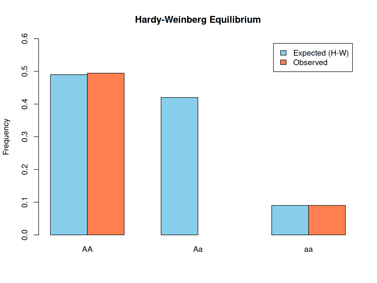
Example: Eliminating a genetic defect (allele frequency p(a) = 0.20)
Assuming Hardy-Weinberg equilibrium: - Genotype frequencies: AA = 0.64, Aa = 0.32, aa = 0.04
Step 1: Genotype all breeding animals Step 2: Do NOT breed aa animals (affected) Step 3: Decision point for Aa carriers: - Aggressive elimination: Don’t breed Aa animals either - Immediate drop in allele frequency to ~0 - But: lose 32% of breeding candidates (may reduce genetic progress for other traits) - Gradual elimination: Breed Aa animals, but avoid Aa × Aa matings - Prevents aa offspring - Allele frequency decreases gradually over generations - Maintains genetic diversity
Strategy C: Exploiting heterozygote advantage
Example: Myostatin mutations for muscling
In some scenarios, heterozygotes are optimal: - +/+: Normal (baseline performance) - +/mh: Increased muscling, normal fertility/calving - mh/mh: Excessive muscling, low fertility, difficult calving
Breeding strategy: - Use +/mh bulls (identified by DNA test) - Mate to +/+ cows - Offspring: 50% +/+ (normal), 50% +/mh (optimal muscling) - Avoid mh/mh offspring entirely
Cost-Benefit Considerations
DNA testing for simply inherited traits is almost always cost-effective when: 1. The trait has economic value (welfare, product quality, registration requirements) 2. Test cost is modest ($20-80 per animal) 3. Results inform breeding decisions (polled, defects) or marketing (coat color)
Example: A $40 polled DNA test on a bull that will sire 5,000 calves costs $0.008 per calf. If dehorning costs $5-10 per animal (labor, pain relief, infection risk), the economic return is enormous.
4.2.4 Population Genetics: Hardy-Weinberg Equilibrium
To understand how allele frequencies change (or don’t change) in populations, we need to introduce a fundamental principle from population genetics: Hardy-Weinberg equilibrium.
The Hardy-Weinberg Principle
For a single locus with two alleles (A and a), if we know the allele frequencies: - p = frequency of A allele - q = frequency of a allele - p + q = 1
Then, under random mating, the genotype frequencies in the next generation will be: - AA: p² - Aa: 2pq - aa: q²
Suppose in a population, the frequency of the black allele (ED) is p = 0.8 and the red allele (e) is q = 0.2.
Under Hardy-Weinberg equilibrium, genotype frequencies are: - EDED = p² = (0.8)² = 0.64 (64% black homozygous) - EDe = 2pq = 2(0.8)(0.2) = 0.32 (32% black heterozygous) - ee = q² = (0.2)² = 0.04 (4% red)
Therefore, 96% of the population is black (EDED + EDe) and 4% is red (ee).
Assumptions of Hardy-Weinberg Equilibrium
The Hardy-Weinberg principle assumes: 1. Random mating (no assortative mating, no inbreeding) 2. No selection (all genotypes have equal fitness) 3. No mutation (alleles don’t change) 4. No migration (no gene flow between populations) 5. Large population size (no genetic drift)
In real livestock populations, these assumptions are often violated: - Selection is the goal of breeding programs - Inbreeding occurs (especially in purebred populations) - Population size can be small (especially in nucleus herds)
However, Hardy-Weinberg provides a useful baseline for predicting genotype frequencies and understanding how selection changes populations.
Selection Changes Allele Frequencies
When selection acts on a simply inherited trait, allele frequencies change rapidly.
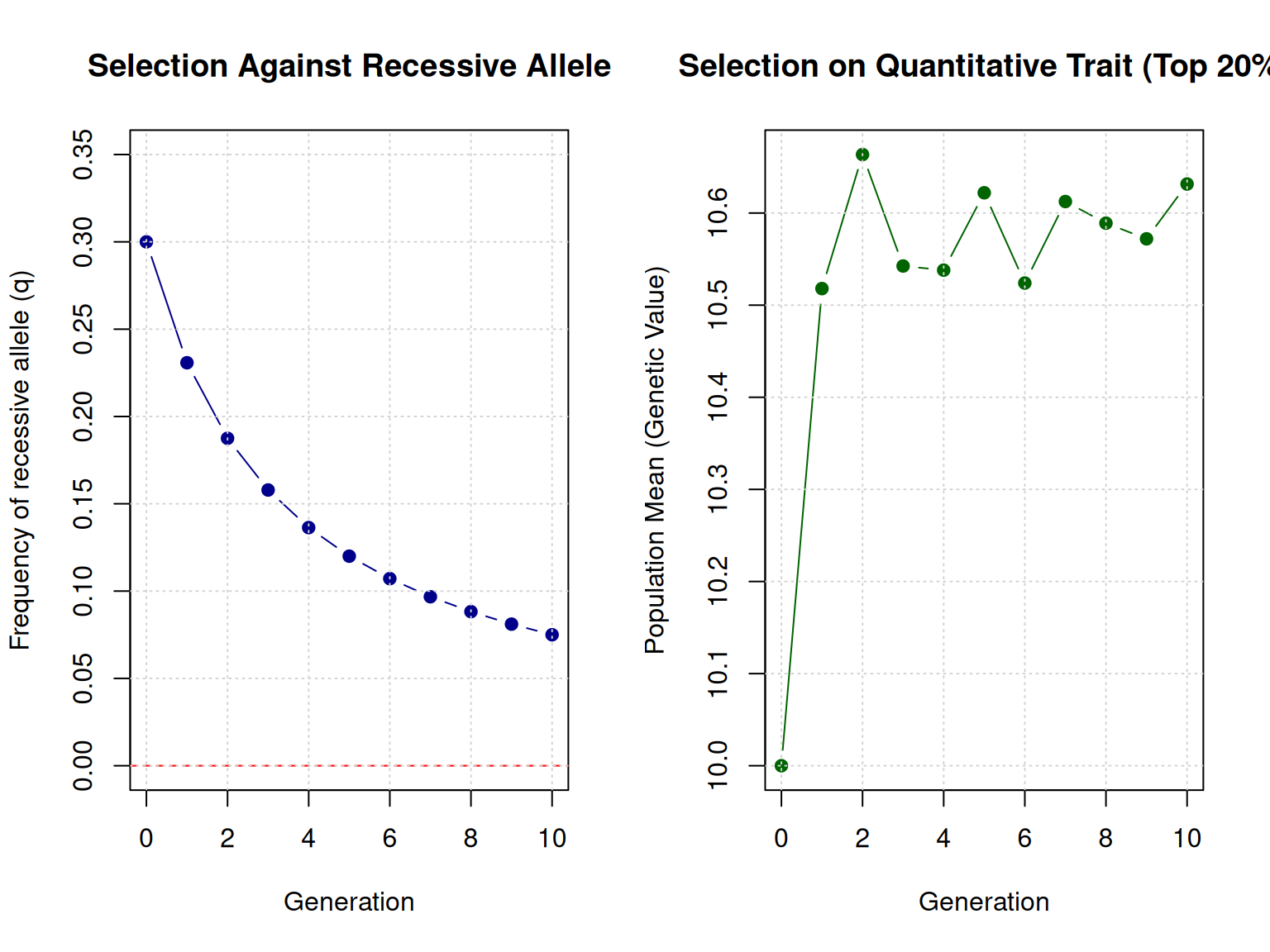
Example: Selecting against a recessive allele
Starting conditions: - q₀ = 0.20 (frequency of recessive allele a) - p₀ = 0.80 (frequency of dominant allele A) - Genotype frequencies (Hardy-Weinberg): AA = 0.64, Aa = 0.32, aa = 0.04
Strategy: Do not breed aa animals (complete selection against aa)
After one generation of selection: - Only AA and Aa animals reproduce - New allele frequencies are calculated from the breeding population - p₁ and q₁ change based on which genotypes contributed offspring
The exact change depends on the selection strategy, but the key point is: simply inherited traits respond quickly to selection because we can directly target specific genotypes.
We’ll explore this more in the R demonstrations section, where we’ll simulate allele frequency changes under different selection scenarios.
4.3 Quantitative Traits
While simply inherited traits follow predictable Mendelian ratios, most economically important livestock traits do not. Milk yield in dairy cattle, growth rate in swine, egg production in layers, and litter size in all species show continuous variation—a smooth distribution of phenotypic values rather than discrete categories. An animal doesn’t produce “high milk yield” or “low milk yield” as distinct categories; instead, cows produce 5,000 kg, 10,000 kg, 15,000 kg, or anywhere in between.
These traits are called quantitative traits (or polygenic traits) because they are influenced by many genes (poly = many), each contributing a small effect. Rather than one gene determining the entire phenotype, hundreds or thousands of genetic variants across the genome each nudge the phenotype up or down slightly. The cumulative effect of all these small genetic effects, combined with environmental influences, produces the continuous distributions we observe.
For quantitative traits: - We cannot predict exact offspring phenotypes from parent genotypes - Selection produces gradual improvement over many generations - We need statistical and quantitative methods to estimate genetic merit - Environmental effects often mask genetic differences
Understanding quantitative traits is the foundation of modern animal breeding. Most traits we care about—production, reproduction, health, efficiency—fall into this category. The remainder of this book focuses primarily on methods for improving quantitative traits, starting with the concepts we introduce here.
4.3.1 Characteristics
Quantitative traits share several key features that distinguish them from simply inherited traits:
1. Polygenic inheritance
Quantitative traits are controlled by many genes, often hundreds or thousands. For example: - Milk production in dairy cattle: Genome-wide association studies (GWAS) have identified hundreds of chromosomal regions associated with milk yield, each explaining <1-2% of genetic variation - Growth rate in poultry: Similar story—many small-effect loci across the genome - Litter size in swine: Even more complex, involving maternal genetics, ovulation rate, uterine capacity, embryonic survival
Each gene contributes a small effect (often too small to detect individually), but together they sum to produce substantial genetic variation. This is fundamentally different from simply inherited traits, where one or two genes explain most or all of the phenotypic variation.
2. Continuous phenotypic distributions
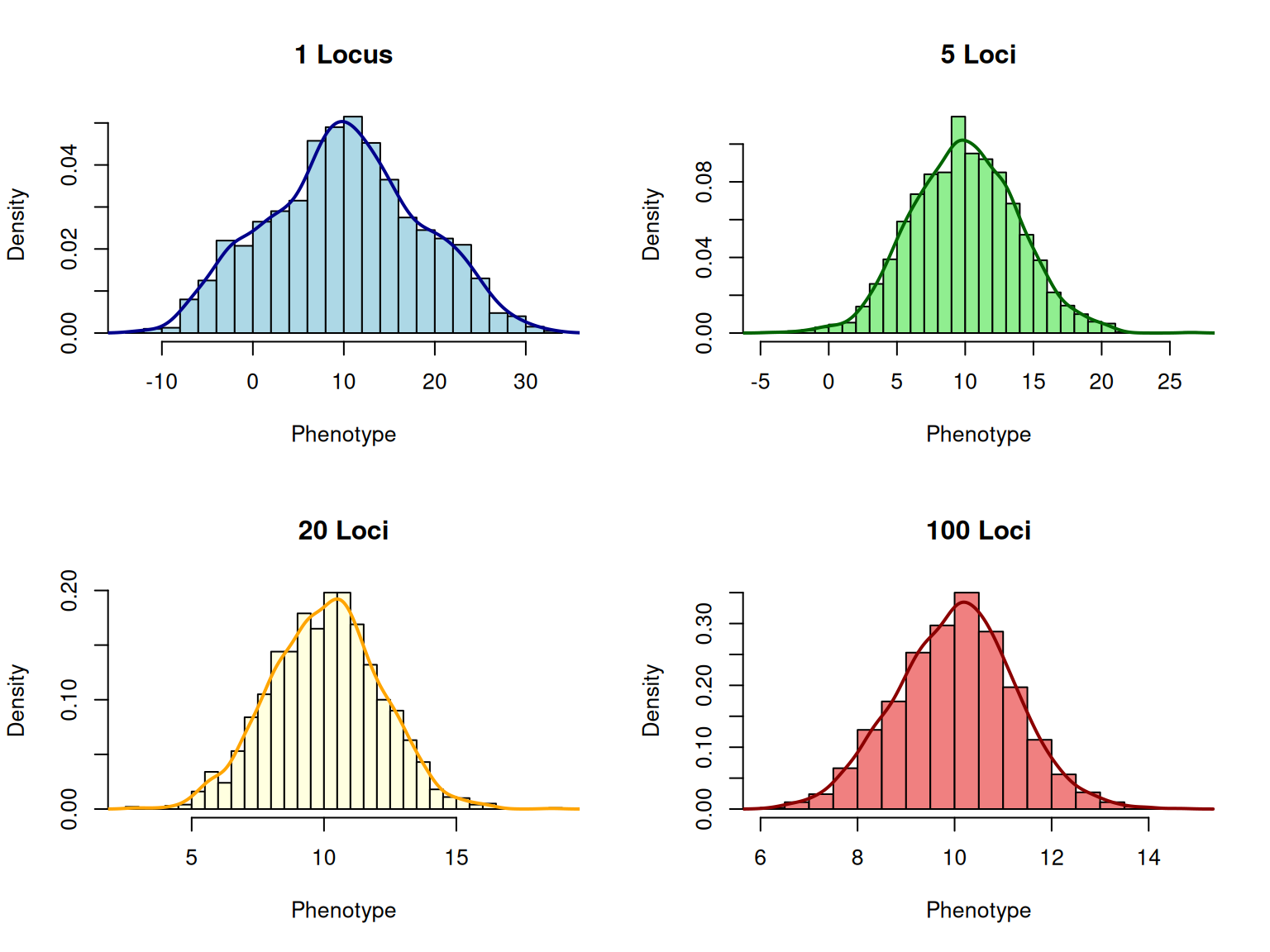
When you plot phenotypes for quantitative traits, you get a smooth, bell-shaped (normal) distribution. This is a consequence of many genes acting additively:
Imagine a trait controlled by 100 genes, each with two alleles (+1 or 0 effect). An individual could inherit: - 0 favorable alleles (phenotype ≈ 0) - 50 favorable alleles (phenotype ≈ 50) - 100 favorable alleles (phenotype ≈ 100) - Or any number in between (1, 2, 3, …, 99)
The most common outcome is around the middle (50 favorable alleles), with fewer individuals at the extremes. This produces the characteristic bell curve (normal distribution).
Environmental effects add additional variation on top of the genetic variation, further smoothing the distribution.
3. Low predictability of offspring phenotypes
Because quantitative traits are influenced by many genes and environment, we cannot precisely predict offspring phenotypes from parent phenotypes or genotypes. For example: - Two parents with above-average milk production will tend to have daughters with above-average milk production - But individual daughters will vary widely around the parental average - Some daughters will be exceptional, others disappointing
This uncertainty makes breeding quantitative traits much more challenging than simply inherited traits. We can only talk about probabilities and expected values, not guaranteed outcomes.
4. Gradual response to selection
Because each gene has a small effect, selection changes allele frequencies slowly at each locus. The population mean shifts gradually over generations: - Fast improvement: High heritability, high selection intensity (e.g., broiler body weight: +50-100 g/year) - Slow improvement: Low heritability, moderate selection intensity (e.g., dairy cow fertility: small gains per year)
Contrast this with simply inherited traits, where a desirable allele can go from rare to common in just 2-3 generations.
5. Strong environmental influence
Quantitative traits are typically influenced substantially by environment: - Management (nutrition, housing, health) - Year and season effects (temperature, humidity, disease pressure) - Contemporary group (herd, flock, pen)
For simply inherited traits, environment may affect expression slightly (e.g., coat color intensity) but doesn’t change the underlying genotype. For quantitative traits, environmental effects can be as large or larger than genetic effects, making it critical to account for environment when estimating genetic merit.
6. Require statistical methods
Because of the complexity of quantitative traits, we need sophisticated statistical methods to: - Partition phenotypic variation into genetic and environmental components - Estimate breeding values (genetic merit) for each animal - Predict genetic change from selection - Design optimal selection strategies
These methods—heritability, breeding values, selection indices, BLUP, genomic selection—are the core tools of quantitative genetics and the focus of Chapters 5-13.
4.3.2 The Three Pillars of Quantitative Genetics
Before diving into specific livestock examples, it’s worth stepping back to understand the conceptual foundations of quantitative genetics. The field rests on three fundamental observations about quantitative traits. These “three pillars” explain why quantitative genetics works and provide the rationale for all the breeding methods we’ll discuss in later chapters.
Pillar 1: Relatives Resemble Each Other
The first pillar is that relatives resemble each other for quantitative traits more than unrelated animals do.
Why? Because relatives share genes. The more closely related two animals are, the more genes they share, and therefore the more similar their phenotypes tend to be (on average).
Examples: - Daughters of high-producing dairy cows tend to be high-producing themselves - Full siblings (same sire and dam) are more similar than half-siblings (same sire, different dams) - Offspring of fast-growing broilers tend to grow faster than offspring of slow-growing broilers
Key insight: If traits had no genetic basis, relatives would be no more similar than unrelated animals. The fact that they are more similar tells us that genetics matters. The degree of resemblance quantifies how much genetics matters—this is the basis for heritability (Chapter 5).
Connection to breeding: Because relatives resemble each other, we can predict an animal’s genetic merit by measuring: - Its own performance - Its parents’ performance - Its siblings’ performance - Its offspring’s performance
This is the foundation for breeding value estimation (Chapter 7).
Pillar 2: Populations Respond to Selection
The second pillar is that populations change in response to selection.
Why? Because selection changes allele frequencies. When we preferentially breed animals with higher phenotypic values, we’re indirectly increasing the frequency of alleles that increase the trait. Over generations, favorable alleles become more common, and the population mean shifts upward.
Examples: - 60+ years of selection on broiler chickens has increased body weight at 6 weeks from ~1 kg to ~3 kg - Dairy cattle milk production has doubled in the past 50 years through systematic selection - Selection for reduced backfat in swine has decreased backfat depth from ~30 mm to ~10 mm
Key insight: The magnitude of response depends on: - How much genetic variation exists (more variation → more response) - How accurately we identify superior animals (better selection → more response) - How intensely we select (fewer parents selected → more response) - How quickly generations turn over (faster generations → faster response)
Connection to breeding: This pillar tells us that genetic improvement is possible and predictable. The breeder’s equation (Chapter 6) formalizes how much response to expect from selection.
Pillar 3: Phenotypic Variation Can Be Partitioned into Components
The third pillar is that we can statistically decompose phenotypic variation into genetic and environmental components.
Recall from Chapter 3 that the basic genetic model for a quantitative trait is:
y = μ + A + E
where: - y = observed phenotype - μ = population mean - A = additive genetic effect (breeding value) - E = environmental deviation
Taking variances of both sides (assuming A and E are independent):
σ²P = σ²A + σ²E
where: - σ²P = phenotypic variance (total variation we observe) - σ²A = additive genetic variance (variation due to breeding values) - σ²E = environmental variance (variation due to environment)
Why this matters: This decomposition allows us to quantify: - How much of the differences we see between animals are genetic vs. environmental - How much genetic improvement is possible - How reliably we can predict offspring performance from parents
Key insight: The ratio σ²A / σ²P is heritability (h²), one of the most important parameters in animal breeding. High heritability means genetics explains most of the phenotypic variation, so selection will be highly effective. Low heritability means environment explains most of the variation, so selection must be more sophisticated (more animals measured, better environmental control, genomic information).
Connection to breeding: Heritability determines: - How similar offspring will be to their parents (regression of offspring on parent = h²/2) - How much response to expect from selection - How accurately we can estimate breeding values
The Three Pillars Work Together
These three pillars are interconnected:
Resemblance between relatives (Pillar 1) exists because of shared genetic variance (Pillar 3)
Response to selection (Pillar 2) occurs because selection changes the genetic component (Pillar 3) of the phenotype
We can predict response to selection (Pillar 2) using estimates of resemblance between relatives (Pillar 1)
Throughout the rest of this book, we’ll repeatedly return to these pillars. They provide the conceptual foundation for heritability, breeding value estimation, selection response, and all modern breeding methods.
4.3.3 Fisher’s Infinitesimal Model
A natural question arises: If quantitative traits are controlled by hundreds or thousands of genes, how can we possibly predict the genetic merit of animals or the response to selection? The answer lies in a brilliant insight by R.A. Fisher in 1918, called the infinitesimal model.
The Infinitesimal Model
Fisher proposed that for quantitative traits: 1. The trait is influenced by a very large number of genes 2. Each gene has a very small effect 3. The genes act additively (no dominance or epistasis, or these effects are small) 4. The environmental effects are also numerous and add to the genetic effects
Under these assumptions, even though we can’t track individual genes, the sum of all genetic effects (the breeding value, A) behaves in a predictable, normally distributed way. This is a consequence of the Central Limit Theorem from statistics, which says that the sum of many independent random variables (in this case, allele effects) follows a normal distribution.
Why this is powerful:
We don’t need to know which genes affect the trait or what their individual effects are. We can treat the breeding value (A) as a single random variable with: - Mean = μA (population mean breeding value, often set to 0) - Variance = σ²A (additive genetic variance)
Similarly, the environmental effects (E) can be treated as: - Mean = 0 - Variance = σ²E (environmental variance)
Practical consequences:
The infinitesimal model allows us to: - Estimate heritability (h² = σ²A / σ²P) without knowing individual genes - Predict breeding values using phenotypes and pedigrees (BLUP) - Calculate expected response to selection (breeder’s equation) - Use genomic selection to capture effects of many small-effect genes
Is the infinitesimal model realistic?
Modern genomics has revealed that real traits are more complex than the infinitesimal model assumes: - Some genes have moderate-to-large effects (not infinitesimal) - Dominance and epistasis exist - Gene effects are not always additive
However, for most quantitative traits in livestock, the infinitesimal model is a remarkably good approximation. Traits like milk yield, growth rate, and litter size do appear to be influenced by hundreds of loci, each with small effects. Even when a few large-effect loci exist (e.g., DGAT1 for milk fat percentage, myostatin for muscling), the infinitesimal model still works well for the remaining polygenic component.
Modern genomic methods (Chapter 13) extend the infinitesimal model by: - Allowing genes to have different variances (some larger, some smaller) - Capturing linkage disequilibrium between markers and QTL - Using hundreds of thousands of SNP markers to approximate the infinitesimal genetic architecture
Fisher’s infinitesimal model remains the conceptual foundation of animal breeding more than a century after it was proposed.
4.3.4 Examples in Livestock
Now let’s examine specific quantitative traits across livestock species. For each trait, we’ll note typical heritability values (h²), which quantify the proportion of phenotypic variance due to additive genetics. We’ll define heritability formally in Chapter 5, but for now, interpret h² as: - h² close to 0: Little genetic variation, slow response to selection - h² around 0.30-0.40: Moderate genetic variation, good response to selection - h² above 0.50: High genetic variation, rapid response to selection
Growth and Feed Efficiency
Average Daily Gain (ADG)
Average daily gain measures how quickly animals grow from birth to market weight. It’s one of the most economically important traits across livestock species.
Species examples: - Swine: ADG from weaning to market (typically 0.7-1.0 kg/day) - h² ≈ 0.30-0.40 (moderate to high heritability) - 50+ years of selection has increased ADG by ~50% - Industry example: PIC/Genus selects intensely for ADG in terminal sire lines
Beef cattle: ADG during feedlot period (typically 1.0-1.8 kg/day)
h² ≈ 0.35-0.50 (high heritability)
One of the most heritable traits in beef cattle
EPDs for yearling weight strongly correlated with ADG
Broilers: Body weight at processing age (35-42 days)
h² ≈ 0.30-0.40 (moderate to high heritability)
Spectacular response to selection: body weight at 6 weeks increased from ~1 kg (1950s) to ~3 kg (2020s)
Companies like Cobb and Aviagen select across multiple genetic lines
Why ADG is highly heritable: Growth rate integrates many physiological processes (appetite, digestion, metabolism, muscle development), but these processes show substantial genetic variation. Environmental factors matter (nutrition, health, housing), but differences between animals in the same environment are largely genetic.
Residual Feed Intake (RFI)
RFI is a measure of feed efficiency independent of growth rate and body size. It’s calculated as:
RFI = Actual feed intake - Expected feed intake (based on growth and maintenance)
Animals with negative RFI eat less than expected (more efficient). Animals with positive RFI eat more than expected (less efficient).
Species examples: - Beef cattle: RFI during feedlot test period - h² ≈ 0.30-0.40 (moderate heritability) - Difference of 1 SD in RFI = ~200-300 kg less feed consumed over lifetime - Major focus for improving sustainability and profitability
Genomic selection makes RFI economically viable to improve
Industry application: RFI is expensive to measure phenotypically (requires individual feed intake monitoring with GrowSafe, FIRE, or similar systems). However, genomic selection (Chapter 13) allows breeding companies to select for RFI by genotyping candidates and using reference populations with measured RFI. This has been a major success story for genomics in livestock.
Reproductive Performance
Reproductive traits are among the most economically important but also the most challenging to improve. They typically have low heritability (h² < 0.20) because: - Complex physiological processes (ovulation, fertilization, embryo development, parturition) - Strongly influenced by environment (nutrition, stress, disease, management) - Subject to natural selection (fertility is a fitness trait)
Litter Size in Swine
Total number born (TNB) or number born alive (NBA) per litter is critical for swine profitability.
Typical values: 11-14 pigs born alive per litter (modern commercial sows)
Why improvement has been slow: Despite intense selection for 50+ years, genetic progress for litter size has been modest (~0.1-0.2 pigs per litter per decade). The low heritability means: - Individual sow records are not highly predictive - Need progeny testing (expensive and slow) or genomic selection - Environmental noise makes identifying genetically superior animals difficult
Industry approach: - Select on estimated breeding values (EBVs) combining own, dam, and maternal granddaughter records - Use genomic selection to increase accuracy - Maternal line indices heavily weight litter size (20-40% of total index)
Daughter Pregnancy Rate in Dairy Cattle
Fertility in dairy cattle has declined over the past 30-40 years, correlated with intense selection for milk production (antagonistic genetic correlation, Chapter 8).
h² ≈ 0.03-0.05 (very low heritability)
Measures the probability a cow becomes pregnant in a 21-day period
Includes both ovulation and conception
Industry response: Modern selection indices (e.g., Net Merit in the US) now include fertility traits with substantial economic weight to counteract the negative correlation with milk yield. Genomic selection has increased accuracy for low-heritability fertility traits, enabling modest genetic improvement.
Age at Puberty in Beef Cattle
Earlier puberty in replacement heifers is economically desirable (younger age at first calving, longer productive life).
h² ≈ 0.30-0.50 (moderate to high heritability)
Can be measured as age at first estrus or scrotal circumference in bulls (correlated)
Scrotal circumference is commonly used as an indicator trait (easier to measure)
Industry approach: Breed associations (e.g., American Angus Association) include scrotal circumference EPDs in maternal breeding indices. Selecting bulls with larger scrotal circumference indirectly improves daughter fertility.
Production Traits
Milk Yield and Components (Dairy Cattle)
Milk production traits are the cornerstone of dairy cattle breeding.
Historical genetic progress: - Milk yield has increased ~100-150 kg per lactation per year over the past 30 years - In the genomic era (post-2009), rate of gain has doubled - Average US Holstein now produces ~11,000-12,000 kg per lactation (up from ~6,000 kg in the 1970s)
Industry structure: Dairy cattle breeding is dominated by AI organizations (Select Sires, ABS Global, CRV, Semex, Alta Genetics). These companies: - Maintain elite bull studs - Collect and process semen for global distribution - Implement genomic selection (testing thousands of young bulls annually) - Market bulls based on genomic estimated breeding values (GEBVs)
Egg Production (Layers)
Egg production and egg quality traits are key for layer breeding.
Traits and heritabilities: - Egg number (eggs per hen to 72 weeks): h² ≈ 0.25-0.35 (moderate) - Egg weight (g): h² ≈ 0.50-0.60 (high) - Shell strength (breaking strength or deformation): h² ≈ 0.30-0.50 (moderate to high) - Internal egg quality (albumen height, yolk color): h² ≈ 0.20-0.40 (moderate)
Genetic correlations: - Egg number and egg weight are negatively correlated (rA ≈ -0.3 to -0.4) - Selection for more eggs tends to reduce egg size, requiring balanced selection
Industry approach: Layer breeding is controlled by a few multinational companies (Hy-Line International, ISA/Hendrix Genetics, Lohmann Breeders). Breeding programs: - Use highly structured pedigree populations (closed nucleus) - Short generation intervals (9-12 months) - Family-based selection with genomic information - Separate brown-egg and white-egg lines
Why carcass traits have high heritability: Carcass composition reflects relatively simple biological processes (muscle and fat deposition) with substantial genetic control and less environmental “noise” than reproduction or health traits.
Industry application: Ultrasound technology allows measurement of carcass traits on live animals, enabling selection before slaughter. Terminal sire indices for beef and swine place heavy emphasis on carcass traits (30-50% of total index weight).
Health and Fitness
Disease Resistance
Improving disease resistance through genetic selection is increasingly important for animal welfare, reducing antibiotic use, and improving productivity.
Examples: - Mastitis resistance in dairy cattle: h² ≈ 0.05-0.15 (low) - Measured indirectly via somatic cell score (SCS) - Included in selection indices (Net Merit includes SCS)
PRRS resistance in swine: h² ≈ 0.10-0.30 (low to moderate)
Porcine Reproductive and Respiratory Syndrome, major disease
Genomic selection used to improve resistance
Gene editing (CD163 knockout) under development
Coccidiosis resistance in chickens: h² ≈ 0.15-0.30 (moderate)
Can be measured by challenge tests
Breeding for resistance reduces reliance on anticoccidial drugs
Challenge: Measuring disease resistance is difficult: - Requires disease challenge or field outbreak data - Health events are binary (sick/not sick), complicating analysis - Low frequency of disease in well-managed herds reduces data availability
Genomic selection impact: Disease resistance traits benefit greatly from genomic selection because phenotyping is expensive and difficult, but genotyping is cheap and accurate.
Longevity and Stayability
Longevity (productive life span) is economically important because: - Longer-lived animals amortize replacement costs over more production cycles - Reduce the proportion of the herd in the replacement phase - Often correlated with overall fitness and health
Dairy cattle productive life: - h² ≈ 0.10-0.20 (low to moderate) - Measured as months of productive life or probability of surviving to 6 years - Included in Net Merit index
Beef cattle stayability: - h² ≈ 0.15-0.25 (moderate) - Measured as probability a cow stays in herd to 6 years of age - Indicator of fertility, udder soundness, structural correctness
Sow longevity in swine: - h² ≈ 0.10-0.15 (low) - Critical for sow productivity (amortize gilt cost over more litters) - Maternal line indices include longevity
Leg Soundness
Skeletal and leg problems reduce welfare and productivity, especially in fast-growing species.
Broilers: - Leg problems (tibial dyschondroplasia, valgus/varus deformities) - h² ≈ 0.10-0.30 (low to moderate) - Genetically correlated with body weight (faster growth = more leg problems) - Breeding companies include leg scoring in selection indices
Layers in cage-free systems: - Keel bone damage (fractures, deviations) - Emerging trait as industry shifts to alternative housing - h² ≈ 0.10-0.40 (varies by specific measure)
Dairy cattle: - Foot and leg conformation scores - h² ≈ 0.10-0.20 (low to moderate) - Included in type/conformation indices
Balancing production and soundness: High-producing animals often have more health and soundness issues due to genetic correlations and metabolic stress. Modern breeding programs must balance production with fitness traits using multi-trait selection indices (Chapter 9).
4.3.5 Why Most Economic Traits are Quantitative
You might wonder: if simply inherited traits are so much easier to manage, why aren’t more economically important traits controlled by single genes? The answer lies in the biological complexity of production, reproduction, and fitness traits.
Complex traits involve many physiological systems
Consider milk production in dairy cattle. To produce milk, a cow must: 1. Consume and digest feed (appetite, rumen function, nutrient absorption) 2. Partition nutrients to mammary gland (metabolism, hormone signaling) 3. Synthesize milk components (protein synthesis, fat synthesis, lactose synthesis) 4. Maintain milk secretion over lactation (mammary cell function, hormone regulation) 5. Support body maintenance (immune function, thermoregulation, reproduction)
Each of these processes involves dozens of genes encoding enzymes, receptors, transporters, structural proteins, and regulatory factors. Variation in any of these genes can affect milk yield. Therefore, milk yield is inevitably polygenic.
Similarly: - Growth requires coordinated regulation of appetite, digestion, nutrient partitioning, protein synthesis, bone development, and metabolism - Reproduction involves ovarian function, hormone cycles, embryo development, uterine receptivity, and maternal care - Disease resistance involves innate immunity, adaptive immunity, inflammation, and physiological resilience
No single gene can control complex processes
For a single gene to control a complex trait, it would need to: - Regulate all the pathways involved in that trait - Have large effects without causing detrimental side effects in other processes
Such “master regulatory genes” are rare. When they do exist (e.g., myostatin for muscle development), they often have undesirable pleiotropic effects (e.g., calving difficulty, reduced fertility).
Trade-offs and evolutionary constraints
Many economically important traits are under stabilizing natural selection—that is, intermediate values have been favored over evolutionary time. For example: - Very high growth rates reduce fertility and increase leg problems - Extremely high milk production compromises cow health and longevity - Maximum litter size may exceed uterine capacity, reducing piglet survival
If a major gene variant dramatically increased any of these traits, natural selection would likely act against it due to fitness costs. Therefore, most genetic variation for production traits comes from many genes with small effects that maintain trade-offs.
Mutations with large effects are rare
Beneficial mutations with large effects are intrinsically rare because: - Most large-effect mutations are deleterious (disrupting essential functions) - Large-effect alleles are quickly fixed or eliminated by natural or artificial selection - Ongoing polygenic variation comes from many small-effect alleles maintained by mutation-selection balance
Conclusion
The polygenic nature of economically important traits is not an inconvenient accident—it’s a fundamental consequence of biological complexity. Understanding quantitative genetics is therefore essential for animal breeding. The good news is that quantitative genetic methods (heritability, BLUP, genomic selection) allow us to improve these traits systematically, even without knowing the identity or function of individual genes.
4.3.6 Breeding Approaches for Quantitative Traits
Breeding quantitative traits requires fundamentally different strategies than simply inherited traits. We can’t use DNA tests to fix or eliminate alleles (there are too many genes involved). Instead, we must use statistical methods to estimate genetic merit and predict offspring performance.
Step 1: Collect phenotypic data
For quantitative traits, we need extensive phenotypic data: - Own performance records (growth, production, carcass) - Progeny performance (offspring testing for sires) - Sibling performance (family information) - Repeated records (multiple lactations, litters)
The more data we have, the more accurately we can estimate genetic merit.
Step 2: Account for environmental effects
Because quantitative traits are strongly influenced by environment, we must adjust data for non-genetic factors: - Contemporary groups: herd, year, season, pen, flock - Fixed effects: age, sex, parity, management - Systematic trends: genetic trends, year effects
Statistical models (linear mixed models) separate genetic from environmental effects.
Step 3: Estimate breeding values (EBVs)
For each animal, we estimate its breeding value—the sum of its additive genetic effects. Breeding values are expressed as deviations from the population mean: - Positive EBV: genetically superior - Negative EBV: genetically inferior - EBV = 0: average genetic merit
Methods for estimating breeding values: - Own performance: Simple but ignores relatives - Parent average: Uses pedigree but ignores own performance - Progeny testing: Accurate but slow (requires waiting for offspring) - BLUP (Best Linear Unbiased Prediction): Uses all information (own, parents, siblings, progeny) optimally - Genomic selection (GBLUP, ssGBLUP): Uses DNA markers to predict breeding values without phenotypes or progeny
We’ll cover breeding value estimation in detail in Chapter 7.
Step 4: Select based on EBVs
Once we have EBVs, selection is conceptually straightforward: - Rank candidates by EBV (or selection index, Chapter 9) - Select top animals as parents - Mate selected parents
Challenges: - Accuracy: EBVs are predictions with uncertainty - Multiple traits: Must balance improvement across traits (selection indices, Chapter 9) - Genetic diversity: Intense selection risks inbreeding (mating strategies, Chapter 10)
Step 5: Iterate over generations
Unlike simply inherited traits (which can be fixed in 1-3 generations), quantitative traits improve gradually: - Population mean shifts each generation - Genetic variance may decline slowly (selection reduces variation) - Breeding programs continue indefinitely
Industry examples:
Dairy cattle (genomic selection): 1. Genotype young bulls and heifers at birth ($30-50 per animal) 2. Compute genomic EBVs (GEBVs) using reference population with phenotypes 3. Select top bulls for AI use based on GEBVs (no progeny testing) 4. Generation interval reduced from 6-7 years to 2-3 years 5. Rate of genetic gain doubled compared to pre-genomic era
Swine (RFI selection with genomics): 1. Measure individual feed intake on ~2,000-5,000 animals per year (reference population) 2. Genotype all selection candidates (10,000-20,000 animals per year) 3. Compute genomic EBVs for RFI using reference population 4. Select candidates based on multi-trait index including genomic EBV for RFI 5. Achieve genetic gain for expensive-to-measure trait without phenotyping every candidate
Beef cattle (EPDs with genomic enhancement): 1. Collect phenotypes from seedstock herds (growth, carcass) 2. Genotype bulls and heifers ($30-50) 3. Breed associations run single-step GBLUP to compute genomic-enhanced EPDs 4. Seedstock breeders select animals based on EPDs 5. Commercial producers buy bulls based on EPDs relevant to their production system (terminal vs. maternal)
Key principles:
Quantitative trait improvement requires: - Data: Extensive, accurate phenotyping - Genetic evaluation: BLUP or genomic methods - Selection: Sustained, systematic selection on EBVs - Patience: Gradual progress over many generations
The remainder of this book focuses on the tools and methods needed to optimize genetic improvement of quantitative traits.
4.4 Threshold Traits
Some traits appear to be simply inherited—they occur in discrete categories (affected vs. unaffected)—but don’t follow Mendelian ratios. Instead, they behave more like quantitative traits, with continuous genetic variation underlying the categorical phenotypes. These are called threshold traits.
Threshold traits represent an important middle ground between simply inherited and truly quantitative traits. Understanding them is critical for breeding decisions involving reproductive, health, and conformational traits in livestock.
4.4.1 Concept: Liability and Threshold
The liability-threshold model (developed by Sewall Wright and D.S. Falconer) explains how continuous genetic variation can produce categorical phenotypes.
Key idea:
Underlying liability: There is an unobserved, continuous variable called liability (or susceptibility) for the trait
Liability has genetic and environmental components: Like any quantitative trait, liability = genes + environment
Threshold: When an animal’s liability exceeds a certain threshold value, the trait is expressed
where: - μ = mean liability in the population - A = genetic component (breeding value for liability) - E = environmental component
If L > T (threshold), then phenotype = 1 (affected) If L ≤ T (threshold), then phenotype = 0 (normal)
Why this matters:
Even though we observe only 0/1 phenotypes, the underlying liability is heritable just like any quantitative trait. Therefore: - Relatives of affected animals have higher liability (on average) - Selection can reduce the frequency of the trait by shifting population liability downward - We can estimate heritability on the liability scale, even though we observe only categorical data
Heritability on liability scale vs. observed scale:
Liability scale: h²L = proportion of variance in liability due to genetics (typically 0.05-0.40)
Observed scale: h²obs = heritability calculated directly from 0/1 data (always lower than h²L, and depends on trait frequency)
Most genetic evaluations report heritability on the liability scale because it’s biologically more meaningful.
4.4.2 Examples in Livestock
Calving Difficulty (Dystocia) in Cattle
Calving difficulty is scored categorically: - 1 = No assistance - 2 = Easy pull - 3 = Hard pull - 4 = Caesarean section - 5 = Abnormal presentation (malpresentation, dead calf)
Why it’s a threshold trait: Calving difficulty depends on continuous factors: - Calf size (birth weight) - Pelvic area of dam - Calf shape and presentation - Strength of uterine contractions - Gestation length
These factors vary continuously, but the outcome (easy vs. difficult calving) is categorical based on whether the calf can pass through the birth canal.
Genetic parameters: - h²L ≈ 0.10-0.20 (liability scale) - Influenced by both calf genetics (direct effect) and dam genetics (maternal effect)
Breeding approach: - Beef breeds report calving ease EPDs (direct and maternal) - Select bulls with positive direct calving ease EPDs for use on heifers - Reduce birth weight while maintaining growth (genetic correlation of +0.50-0.70)
Teat Number and Inverted Teats in Swine
Piglets need sufficient functional teats to nurse. Defects include: - Inverted teats (non-functional) - Fewer than 12-14 teats total
Why it’s a threshold trait: Teat development during embryogenesis involves continuous developmental processes. When these processes are disrupted beyond a threshold, inverted or missing teats result.
Genetic parameters: - h²L ≈ 0.10-0.30 for teat number (liability scale) - Frequency of inverted teats: 5-15% in some lines
Breeding approach: - Visually score gilts and boars for teat defects - Cull animals with inverted teats or fewer than 12 teats - Include teat score in maternal line selection indices - Genomic selection can improve accuracy despite categorical scoring
Retained Placenta in Dairy Cattle
Retained placenta (failure to expel fetal membranes within 12-24 hours after calving) is a categorical trait (yes/no) but with continuous underlying liability.
Factors affecting liability: - Immune function - Uterine health - Calving difficulty - Nutritional status (especially calcium, vitamin E, selenium) - Gestation length
Genetic parameters: - h²L ≈ 0.05-0.10 (low heritability on liability scale) - Frequency: 5-15% of calvings
Breeding approach: - Direct selection is difficult (low heritability, confounded with environment) - Correlated selection through calving ease and immune function traits - Modern selection indices include calving and health traits
Twinning in Cattle
In most cattle breeds, twinning is undesirable (increased calving difficulty, lower calf survival, reduced subsequent fertility). However, twinning behaves as a threshold trait with underlying genetic liability.
Genetic parameters: - h²L ≈ 0.05-0.15 - Twinning rate: typically 1-5% in single-birth breeds, higher in breeds selected for twinning
Breeding approach: - Most breeds select against twinning - Some specialized breeding programs have selected for twinning to increase reproductive efficiency (requires specialized management)
4.4.3 Genetic Analysis of Threshold Traits
Estimating heritability on the liability scale
Given: - p = frequency of affected individuals (proportion with phenotype = 1) - r = correlation between relatives (parent-offspring, full sibs, half sibs) for the categorical trait
We can estimate h²L using transformations based on the normal distribution. The key insight is that if liability is normally distributed, we can infer the distribution parameters from the observed frequency.
Example calculation:
Suppose calving difficulty (coded as difficult = 1, normal = 0) has frequency p = 0.10 (10% of calves require assistance). The correlation between dam and daughter for calving difficulty is r = 0.05.
From statistical tables (or software), when p = 0.10, the transformation factor is approximately 1.7.
This tells us that ~8.5% of variance in liability is genetic.
Breeding value estimation:
Modern genetic evaluation programs can analyze threshold traits using: - Linear models on observed scale: Simple but biased - Threshold mixed models: Explicitly model liability scale using Bayesian MCMC methods - Genomic approaches: Genomic selection treats liability as quantitative
Many breed associations use threshold models for traits like calving ease to more accurately estimate breeding values.
Response to selection:
Because threshold traits have underlying quantitative liability, selection works, but response depends on: - Heritability on liability scale (h²L) - Trait frequency (rare traits have less information) - Selection intensity - Accuracy of liability estimates
Selection shifts the population distribution of liability, reducing the proportion of animals exceeding the threshold. This gradually decreases the frequency of the undesirable phenotype.
4.5 Mixed Model Traits
Most traits don’t fit neatly into “simply inherited” or “quantitative” categories. In reality, many economically important traits have mixed genetic architecture: they’re primarily quantitative (controlled by many small-effect genes) but also influenced by one or a few genes with larger effects. These are called mixed model traits or traits with major QTL (Quantitative Trait Loci).
Understanding mixed model traits is important because: - They’re common in livestock (muscling, disease resistance, milk composition) - They require different breeding strategies than purely polygenic traits - Modern genomics can identify and exploit major QTL
4.5.1 Characteristics
Mixed model traits combine features of both simply inherited and quantitative traits:
Quantitative background: - Continuous phenotypic distribution - Influenced by many small-effect genes (polygenic component) - Responds to selection gradually
Plus major gene effects: - One or a few loci with moderate to large effects - These loci explain 5-30% of genetic variance (much more than typical SNPs) - Can be detected through genome-wide association studies (GWAS) - May have functional mutations identified (e.g., DGAT1 for milk fat, RYR1 for halothane)
Genetic model:
y = μ + M + Apoly + E
where: - y = phenotype - μ = population mean - M = major gene effect (one or few large-effect loci) - Apoly = polygenic effect (many small-effect loci) - E = environmental effect
The major gene (M) can be genotyped directly (if mutation is known) or captured by linked SNP markers (in genomic selection).
4.5.2 Example: Halothane Sensitivity and Meat Quality in Swine
As discussed earlier in this chapter, the RYR1 gene causes halothane sensitivity (porcine stress syndrome). But it’s not just a simple genetic defect—it also affects quantitative traits like growth rate and meat quality.
Key observations: - The halothane allele (n) increases lean growth and reduces backfat (desirable) - But it also increases pale, soft, exudative (PSE) meat and transport mortality (undesirable) - The effect is additive to codominant (het
erozygotes intermediate)
Mixed genetic architecture: - Growth rate and carcass composition are polygenic (hundreds of loci) - But RYR1 explains ~5-10% of genetic variance in these traits (a major QTL) - Other genes contribute smaller effects
Historical breeding strategy: - 1960s-1980s: Some lines selected for halothane allele (increased lean) - 1990s-2000s: Industry eliminated halothane allele (welfare and meat quality concerns) - DNA testing allowed rapid elimination within 5-10 years
Modern approach: - Halothane eliminated from most commercial lines - Continued selection for lean growth through genomic selection (captures polygenic effects) - Net result: comparable or better carcass merit without halothane-related problems
4.5.3 Example: DGAT1 and Milk Composition in Dairy Cattle
The DGAT1 (Diacylglycerol O-Acyltransferase 1) gene on chromosome 14 in cattle encodes an enzyme involved in fat synthesis. A single nucleotide polymorphism (K232A mutation) has large effects on milk composition.
Alleles: - K allele (lysine at position 232): Higher fat percentage, lower protein percentage, lower milk yield - A allele (alanine): Lower fat percentage, higher protein percentage, higher milk yield
Effects on milk traits:
Trait
KK
KA
AA
Milk yield (kg/lactation)
9,000
9,500
10,000
Fat percentage (%)
4.3
4.0
3.7
Fat yield (kg/lactation)
387
380
370
Protein percentage (%)
3.3
3.4
3.5
Protein yield (kg/lactation)
297
323
350
Mixed genetic architecture: - Milk yield, fat %, and protein % are highly polygenic (hundreds of loci) - But DGAT1 explains ~3-5% of genetic variance (a major QTL) - Other QTL exist but have smaller effects
Breeding implications: - DGAT1 genotype is included in genomic evaluations - Selection indices can optimize allele frequency based on economic weights - If paid for fat yield: K allele may be favorable - If paid for protein yield or milk volume: A allele is favorable - Most modern genomic evaluations incorporate DGAT1 automatically (captured by nearby SNPs)
4.5.4 Example: Myostatin and Muscling
We discussed myostatin earlier as a simply inherited trait causing double muscling in homozygotes. But in most populations, myostatin mutations are rare or absent, and muscling is quantitative. However, when the mutation is segregating, it acts as a major QTL within an otherwise polygenic trait.
Mixed architecture: - Muscle mass is polygenic (hundreds of loci affect growth, muscle fiber number, metabolism) - But MSTN loss-of-function alleles have huge effects (20-30% increase in muscle) - Breeders must balance major gene effects with polygenic background
Breeding strategy: - In breeds without myostatin mutations: select on EBVs for muscling (purely polygenic) - In breeds with myostatin mutations: use DNA test + EBVs (mixed model) - Genomic selection captures both major and polygenic effects simultaneously
4.5.5 Modern Genomics Approach to Mixed Model Traits
Challenge:
Traditional quantitative genetics methods assume all genes have small, equal effects (infinitesimal model). When major QTL exist, this assumption is violated. How do we handle major genes in genetic evaluations?
Solutions:
1. Explicit inclusion of major gene genotypes
If the causal mutation is known (e.g., RYR1, DGAT1), include genotype as a fixed or random effect in the breeding value estimation model:
EBV = Major gene effect + Polygenic EBV
This separates the major gene from the polygenic background.
2. Genomic selection (captures major and minor effects)
Genomic selection using high-density SNP panels automatically captures major QTL effects: - SNPs in linkage disequilibrium with major QTL get large estimated effects - Other SNPs get small estimated effects - No need to know which genes are major in advance
Methods: - GBLUP: Assumes all SNPs have equal variance (works well even with some large-effect loci) - BayesB, BayesC, Bayesian Lasso: Allow SNPs to have different variances (better for traits with major QTL) - Single-step GBLUP: Combines pedigree, phenotypes, and genomic data; handles mixed architecture well
3. Multi-trait genomic models
When major genes affect multiple traits (like DGAT1 or RYR1), multi-trait models: - Capture genetic correlations - Improve accuracy for correlated traits - Allow index selection to balance traits
Industry implementation:
Most modern breeding programs use genomic selection, which handles mixed model traits automatically: - No need to individually test for every known QTL - SNP arrays capture effects of major and minor genes - Breeding values integrate all genetic information
Example: Dairy cattle genomic evaluation
US dairy genomic evaluations (CDCB) use single-step GBLUP: - Incorporates phenotypes from millions of cows - Genotypes from hundreds of thousands of animals - Automatically captures DGAT1, ABCG2, GHR, and other major QTL - Bulls are ranked by genomic EBVs (GEBVs) that include all genetic effects
Advantage:
Breeders don’t need to know or genotype individual QTL—genomic selection handles the entire genome, regardless of genetic architecture.
4.5.6 Practical Implications
When major QTL are segregating in a population:
Genotype for known QTL (if economically justified)
Direct DNA test can inform mating decisions
Useful for major genes with large, well-characterized effects
Use genomic selection
Captures major QTL automatically via linked SNPs
Also captures all polygenic effects
Most cost-effective approach for most traits
Consider interactions
Major genes may interact with genetic background (epistasis)
Optimal allele at major gene may depend on polygenic background
Multi-trait selection balances effects across traits
Transition from major gene to polygenic selection:
Many traits historically influenced by major genes have transitioned to purely polygenic: - Halothane eliminated from swine → now purely polygenic growth/carcass improvement - Polled allele fixed in Angus → focus shifts to other traits - As major alleles are fixed or eliminated, remaining variation is polygenic
This illustrates that genetic architecture is not static—breeding changes allele frequencies, and the “architecture” of remaining variation evolves over time.
4.6 Comparing Simply Inherited and Quantitative Traits
Now that we’ve explored simply inherited traits, quantitative traits, threshold traits, and mixed model traits, let’s summarize the key differences and practical implications for breeding programs.
4.6.1 Comparison Table
Characteristic
Simply Inherited Traits
Quantitative Traits
Threshold Traits
Mixed Model Traits
Genetic basis
Single gene or few genes with major effects
Many genes (hundreds to thousands), each with small effect
Continuous liability, categorical expression
Mostly polygenic + 1-few major QTL
Phenotypic distribution
Discrete categories (no intermediates)
Continuous (normal distribution)
Categorical observed, continuous liability
Continuous, may show modes if major QTL segregating
Heritability
Not applicable (all-or-none genetic determination)
Milk fat % (DGAT1), muscling if myostatin segregating
Examples - swine
Halothane sensitivity (as genetic defect)
Litter size, average daily gain, feed efficiency
Teat defects, hernias
Growth and carcass with halothane (historical)
Examples - poultry
Plumage color, comb type, polydactyly
Body weight, egg production, feed efficiency
Sudden death syndrome, leg disorders
Egg weight and number (mixed architecture)
Examples - sheep
Coat color, horned/polled
Litter size, fleece weight, growth rate
Prolificacy (litter size as threshold)
Muscling (myostatin in Texel)
Typical variance explained by largest locus
100% (single gene determines phenotype)
<1-2% (each locus tiny effect)
<1-2% (polygenic liability)
5-30% (major QTL), rest polygenic
Industry breeding strategy
Genotype and select/eliminate based on test results
Phenotype extensively, estimate EBVs, select on index
Collect categorical data, threshold BLUP or genomic
Genomic selection (captures all effects), optional direct test for major QTL
Cost of genetic evaluation
Low ($20-80 per DNA test)
High (extensive phenotyping, genetic evaluation infrastructure)
Moderate (categorical data easier to collect)
Moderate to high (genomic + phenotyping)
Time to see genetic improvement
Immediate (within 1-2 generations)
Long-term (5-10+ generations for substantial change)
Moderate (frequency declines gradually)
Moderate (major gene fast, polygenic slow)
Risk of unintended consequences
Low (specific gene, specific effect)
Moderate (genetic correlations, trade-offs)
Moderate (correlated with other traits)
Moderate to high (major genes often pleiotropic)
4.6.2 Key Takeaways from the Comparison
1. Genetic architecture drives breeding strategy
The number and effect sizes of genes controlling a trait fundamentally determine: - What data to collect (genotypes vs. phenotypes vs. both) - What methods to use (DNA tests vs. EBVs vs. genomic selection) - How quickly progress can be made - What resources are required
2. Most economically important traits are quantitative or mixed
Production, reproduction, health, and efficiency traits are inherently complex and polygenic. Simply inherited traits (coat color, polled status, genetic defects) are important but not the primary drivers of profitability in most breeding programs.
3. Modern genomics blurs the distinctions
Genomic selection using high-density SNP arrays: - Captures both major and minor gene effects automatically - Increases accuracy for low-heritability quantitative traits - Enables selection for expensive-to-measure traits - Provides a unified framework regardless of genetic architecture
In practice, most modern breeding programs use genomic selection for all traits and supplement with DNA tests for specific major genes when economically justified.
Even though genomics provides a “one size fits all” solution, understanding whether a trait is simply inherited, quantitative, or mixed helps breeders: - Set realistic expectations for rate of improvement - Interpret genomic predictions appropriately - Make informed mating decisions - Communicate with clients and stakeholders
5. Genetic architecture evolves
As breeding programs fix desirable alleles and eliminate undesirable alleles: - Simply inherited traits transition from segregating to fixed (e.g., polled in Angus) - Mixed model traits become purely quantitative (e.g., growth in swine after halothane elimination) - Remaining genetic variation is increasingly polygenic
This means breeding strategies must evolve over time as populations change.
4.7 R Demonstration: Simulating Different Trait Types
Now let’s use R to simulate the different types of genetic architecture we’ve discussed and visualize how they differ. These simulations will help solidify your understanding of simply inherited vs. quantitative traits.
4.7.1 Demonstration 1: Mendelian Crosses and Segregation Ratios
First, let’s simulate a simple monohybrid cross (Aa × Aa) and verify that we get the expected 3:1 phenotypic ratio.
# Simulate F1 x F1 cross (Aa x Aa)# Each parent contributes one allele randomlyset.seed(123)n_offspring<-10000# Large sample to see clear ratios# Function to simulate a single crosssimulate_cross<-function(parent1_genotype, parent2_genotype){# Each parent is c("A", "a") or c("A", "A") or c("a", "a")# Randomly sample one allele from each parentallele_from_parent1<-sample(parent1_genotype, 1)allele_from_parent2<-sample(parent2_genotype, 1)return(c(allele_from_parent1, allele_from_parent2))}# Simulate Aa x Aa crossparent1<-c("A", "a")parent2<-c("A", "a")offspring_genotypes<-replicate(n_offspring, simulate_cross(parent1, parent2), simplify =FALSE)# Convert to genotype strings and determine phenotypesgenotype_strings<-sapply(offspring_genotypes, function(x){paste(sort(x), collapse ="")# Sort so Aa and aA are both "Aa"})# Determine phenotypes (assuming complete dominance: A is dominant)phenotypes<-ifelse(grepl("A", genotype_strings), "Dominant (A_)", "Recessive (aa)")# Calculate frequenciesgeno_table<-table(genotype_strings)pheno_table<-table(phenotypes)cat("Genotype frequencies:\n")
Interpretation: With 10,000 offspring, we see proportions very close to the expected 1:2:1 genotypic ratio and 3:1 phenotypic ratio. This confirms Mendelian inheritance for a simply inherited trait.
4.7.2 Demonstration 2: Hardy-Weinberg Equilibrium
Now let’s verify Hardy-Weinberg equilibrium: given allele frequencies, we can predict genotype frequencies.
# Hardy-Weinberg equilibrium demonstration# Set allele frequenciesp<-0.7# Frequency of A alleleq<-0.3# Frequency of a allelecat("Allele frequencies:\n")
# Simulate a population under random matingn_pop<-10000set.seed(456)# Each individual gets two alleles, sampled with frequencies p and qallele1<-sample(c("A", "a"), n_pop, replace =TRUE, prob =c(p, q))allele2<-sample(c("A", "a"), n_pop, replace =TRUE, prob =c(p, q))# Determine genotypesgenotypes<-paste0(pmin(allele1, allele2), pmax(allele1, allele2))genotype_freqs<-table(genotypes)/n_popcat("Observed genotype frequencies (simulated):\n")
Interpretation: Under random mating, observed genotype frequencies match Hardy-Weinberg predictions almost exactly. This is the baseline expectation when there is no selection, mutation, migration, or drift.
Now let’s simulate quantitative traits controlled by different numbers of loci and observe how the distribution becomes more normal as the number of loci increases.
# Simulate quantitative traits with different numbers of lociset.seed(789)n_individuals<-2000# Function to simulate a polygenic traitsimulate_polygenic_trait<-function(n_loci, n_individuals, allele_freq=0.5,effect_size=1, env_var=1){# Generate genotypes (0, 1, 2 copies of + allele at each locus)genotypes<-matrix(rbinom(n_individuals*n_loci, 2, allele_freq), nrow =n_individuals, ncol =n_loci)# Genetic values (sum of allele effects)genetic_values<-rowSums(genotypes)*effect_size# Add environmental deviationenvironmental_effects<-rnorm(n_individuals, 0, sqrt(env_var))# Phenotypesphenotypes<-genetic_values+environmental_effectsreturn(list(phenotypes =phenotypes, genetic_values =genetic_values))}# Simulate traits with 1, 5, 20, and 100 locitrait_1_locus<-simulate_polygenic_trait(n_loci =1, n_individuals =n_individuals, effect_size =10, env_var =20)trait_5_loci<-simulate_polygenic_trait(n_loci =5, n_individuals =n_individuals, effect_size =2, env_var =5)trait_20_loci<-simulate_polygenic_trait(n_loci =20, n_individuals =n_individuals, effect_size =0.5, env_var =2)trait_100_loci<-simulate_polygenic_trait(n_loci =100, n_individuals =n_individuals, effect_size =0.1, env_var =1)# Plot distributionspar(mfrow =c(2, 2))hist(trait_1_locus$phenotypes, breaks =30, main ="1 Locus", xlab ="Phenotype", col ="lightblue", prob =TRUE)lines(density(trait_1_locus$phenotypes), col ="darkblue", lwd =2)hist(trait_5_loci$phenotypes, breaks =30, main ="5 Loci", xlab ="Phenotype", col ="lightgreen", prob =TRUE)lines(density(trait_5_loci$phenotypes), col ="darkgreen", lwd =2)hist(trait_20_loci$phenotypes, breaks =30, main ="20 Loci", xlab ="Phenotype", col ="lightyellow", prob =TRUE)lines(density(trait_20_loci$phenotypes), col ="orange", lwd =2)hist(trait_100_loci$phenotypes, breaks =30, main ="100 Loci", xlab ="Phenotype", col ="lightcoral", prob =TRUE)lines(density(trait_100_loci$phenotypes), col ="darkred", lwd =2)
Interpretation: As the number of loci increases, the phenotypic distribution becomes smoother and more closely approximates a normal (bell-shaped) distribution. This illustrates the Central Limit Theorem and Fisher’s infinitesimal model: the sum of many small random effects produces a normal distribution.
4.7.4 Demonstration 4: Selection on Simply Inherited vs. Quantitative Traits
Finally, let’s compare how quickly we can change a population through selection on a simply inherited trait vs. a quantitative trait.
# Simulate selection over multiple generationsset.seed(101112)n_generations<-10pop_size<-1000# ---- Selection against a recessive allele (simply inherited) ----# Starting frequency of recessive allele (a) = 0.30q_initial<-0.30q_values_simple<-numeric(n_generations+1)q_values_simple[1]<-q_initialfor(genin1:n_generations){q<-q_values_simple[gen]p<-1-q# Genotype frequencies (Hardy-Weinberg)freq_AA<-p^2freq_Aa<-2*p*qfreq_aa<-q^2# Selection: do not breed aa individuals (complete selection against aa)# New frequencies among breeding populationfreq_AA_breeding<-freq_AA/(freq_AA+freq_Aa)freq_Aa_breeding<-freq_Aa/(freq_AA+freq_Aa)# Calculate new allele frequencyp_new<-freq_AA_breeding+0.5*freq_Aa_breedingq_new<-1-p_newq_values_simple[gen+1]<-q_new}# ---- Selection on a quantitative trait (100 loci) ----# We'll select the top 20% of individuals based on phenotype each generationpop_mean_quant<-numeric(n_generations+1)# Initialize populationallele_freqs<-rep(0.5, 100)# Start with all loci at frequency 0.5pop_mean_quant[1]<-sum(allele_freqs)*2*0.1# Mean genetic valuefor(genin1:n_generations){# Simulate populationtrait_data<-simulate_polygenic_trait(n_loci =100, n_individuals =pop_size, allele_freq =mean(allele_freqs), effect_size =0.1, env_var =1)# Select top 20%selection_threshold<-quantile(trait_data$phenotypes, 0.80)selected<-trait_data$phenotypes>=selection_threshold# Calculate mean genetic value of selected individualsselected_genetic_mean<-mean(trait_data$genetic_values[selected])# Next generation mean (simplified: assume selected mean becomes new population mean)pop_mean_quant[gen+1]<-selected_genetic_mean}# Plot comparisonpar(mfrow =c(1, 2))# Simply inherited traitplot(0:n_generations, q_values_simple, type ="b", pch =19, col ="darkblue", xlab ="Generation", ylab ="Frequency of recessive allele (q)", main ="Selection Against Recessive Allele", ylim =c(0, 0.35))abline(h =0, lty =2, col ="red")grid()# Quantitative traitplot(0:n_generations, pop_mean_quant, type ="b", pch =19, col ="darkgreen", xlab ="Generation", ylab ="Population Mean (Genetic Value)", main ="Selection on Quantitative Trait (Top 20%)")grid()
Simply inherited: q reduced by 0.0225 per generation
cat("Quantitative: mean increased by",round((pop_mean_quant[11]-pop_mean_quant[1])/10, 2), "per generation\n")
Quantitative: mean increased by 0.06 per generation
Interpretation:
Simply inherited trait: The recessive allele frequency drops rapidly from 0.30 to near zero within 10 generations when we completely select against homozygous recessive individuals.
Quantitative trait: The population mean increases gradually and linearly over 10 generations. The rate of improvement depends on heritability, selection intensity, and genetic variation (Breeder’s Equation, Chapter 6).
This demonstrates the fundamental difference in response to selection: simply inherited traits can be fixed or eliminated quickly, while quantitative traits improve gradually but continuously.
4.8 Summary
This chapter has introduced one of the most fundamental distinctions in animal breeding: the difference between simply inherited traits and quantitative traits. Understanding this distinction is essential because it determines how we collect data, analyze genetics, make breeding decisions, and predict genetic progress.
4.8.1 Key Points
Simply Inherited Traits: - Controlled by single genes or few genes with major effects - Discrete phenotypic categories with no intermediates - Follow Mendelian inheritance patterns (3:1, 9:3:3:1 ratios) - High predictability of offspring from parents - Can be rapidly fixed or eliminated (1-3 generations) using DNA tests - Examples: coat color, polled status, genetic defects, myostatin double muscling - Hardy-Weinberg equilibrium predicts genotype frequencies from allele frequencies - Industry uses DNA tests ($20-80/animal) to identify carriers and make mating decisions
Quantitative Traits: - Controlled by many genes (hundreds to thousands), each with small effects - Continuous phenotypic distributions (normal/bell-shaped) - Cannot predict exact offspring phenotypes, only probabilities - Gradual improvement through selection over many generations - Require statistical methods (BLUP, genomic selection) to estimate breeding values - Examples: milk yield, growth rate, litter size, feed efficiency, disease resistance - Most economically important traits are quantitative due to biological complexity
The Three Pillars of Quantitative Genetics:
Relatives resemble each other: The degree of resemblance quantifies heritability
Populations respond to selection: Allele frequencies change, population mean shifts
Phenotypic variation can be partitioned: σ²P = σ²A + σ²E
These pillars provide the conceptual foundation for heritability (Chapter 5), breeding value estimation (Chapter 7), and selection response (Chapter 6).
Fisher’s Infinitesimal Model: - Assumes many genes, each with infinitesimal effect - Breeding values follow a normal distribution (Central Limit Theorem) - Allows prediction of genetic merit and selection response without knowing individual genes - Remarkably accurate for most livestock traits despite simplifying assumptions - Modern genomic methods extend this model by allowing genes to have different variances
Threshold Traits: - Appear categorical but have continuous underlying liability - Liability = genes + environment; when liability > threshold, trait is expressed - Examples: calving ease, teat defects, retained placenta, twinning - Heritability estimated on liability scale (h²L) - Selection shifts liability distribution, reducing frequency of undesirable phenotypes - Analyzed using threshold models or genomic selection
Mixed Model Traits: - Primarily quantitative but with one or few genes having moderate-to-large effects (major QTL) - Examples: milk composition (DGAT1), meat quality (RYR1 in swine), muscling (myostatin) - Major QTL explain 5-30% of genetic variance; remaining variance is polygenic - Genomic selection automatically captures both major and minor gene effects - As major alleles are fixed/eliminated, traits become purely polygenic
Practical Breeding Implications:
Trait Type
Data Needed
Methods
Time to Improvement
Cost
Simply inherited
Genotypes
DNA tests
1-3 generations
Low ($20-80/test)
Quantitative
Phenotypes
BLUP, genomic selection
5-10+ generations
High (extensive phenotyping)
Threshold
Categorical data
Threshold models, genomic
Moderate
Moderate
Mixed model
Genotypes + phenotypes
Genomic selection
Moderate
Moderate to high
Modern Genomic Selection: - Uses high-density SNP panels (50K-600K+ markers) - Captures all genetic effects regardless of architecture - Doubles accuracy for young animals compared to pedigree alone - Enables selection for expensive-to-measure traits (RFI, disease resistance) - Has become the standard approach in dairy, swine, poultry, and increasingly in beef
Why Most Economic Traits are Quantitative: - Production, reproduction, and fitness involve complex physiological systems - Many genes regulate appetite, metabolism, growth, immunity, reproduction - Trade-offs and evolutionary constraints favor polygenic variation - Beneficial large-effect mutations are rare and often have pleiotropic costs
The Path Forward:
Understanding genetic architecture is foundational for the rest of this book: - Chapter 5 formalizes heritability and variance components - Chapter 6 presents the breeder’s equation for predicting selection response - Chapter 7 explains breeding value estimation (BLUP) - Chapter 8 introduces genetic correlations between traits - Chapter 9 covers multi-trait selection indices - Chapters 12-13 dive deep into genomics and genomic selection
Every method we’ll learn builds on the concepts introduced in this chapter: partitioning genetic and environmental effects, estimating breeding values, and predicting response to selection. Whether you’re breeding dairy cattle for milk production, swine for feed efficiency, or poultry for growth rate, these principles apply universally.
4.9 Practice Problems
Work through these problems to test your understanding of the chapter concepts. Hints and brief solutions are provided at the end.
4.9.1 Problem 1: Classifying Traits
Classify each of the following traits as (a) simply inherited, (b) quantitative, (c) threshold, or (d) mixed model. Justify your answer briefly.
Coat color in horses (multiple alleles at MC1R, ASIP loci)
Milk yield (kg/lactation) in dairy cattle
Polled status in cattle
Litter size in swine
Calving ease in beef cattle
Milk fat percentage in dairy cattle (affected by DGAT1 and many other loci)
Backfat depth in swine
Presence/absence of inverted teats in swine
4.9.2 Problem 2: Hardy-Weinberg Calculations
In a population of beef cattle, the frequency of the red coat color allele (e) at the MC1R locus is 0.20, and the frequency of the black allele (ED) is 0.80. Assume the population is in Hardy-Weinberg equilibrium.
Calculate the expected genotype frequencies (EDED, EDe, ee)
If there are 1,000 cattle in the herd, how many would you expect to be red (ee)?
How many black cattle would be carriers for red (EDe)?
4.9.3 Problem 3: Why Litter Size is Quantitative
Litter size in swine is a quantitative trait with low heritability (h² ≈ 0.10-0.15). Explain:
Why litter size cannot be controlled by a single gene (think about the biological processes involved)
Why heritability is low (what sources of variation affect litter size?)
Why genetic improvement for litter size has been slow despite intense selection
4.9.4 Problem 4: Eliminating a Recessive Defect
A beef cattle breeder discovers that 4% of calves in their herd are born with a recessive lethal genetic defect (genotype aa). Assume Hardy-Weinberg equilibrium.
Calculate the frequency of the recessive allele (a) in the population
What proportion of the breeding herd are carriers (Aa)?
Design a breeding strategy using DNA testing to eliminate this defect within 2-3 generations while maintaining genetic diversity for other traits
Calculate the additive genetic standard deviation (σA) for each trait
If you select the top 20% of animals for each trait separately, which trait will show faster genetic progress? Why?
What does this tell you about the importance of heritability for selection response?
4.9.6 Problem 6: Threshold Trait Analysis
Dystocia (difficult calving) in beef cattle occurs in 10% of first-calf heifers. The heritability of dystocia on the liability scale is h²L = 0.15.
Is dystocia best classified as simply inherited, quantitative, or threshold? Why?
If you cull all heifers that experience dystocia and never breed them, will you eliminate dystocia from the population in one generation? Why or why not?
What would be a more practical breeding strategy to reduce dystocia frequency?
4.9.7 Problem 7: Comparing Genetic Architectures
Consider three traits: - Trait A: Controlled by one gene (polled allele in cattle) - Trait B: Controlled by 5 genes with equal effects - Trait C: Controlled by 100 genes with equal effects
Sketch the expected phenotypic distribution for each trait (assume no environmental effects)
Which trait(s) would show a continuous distribution?
For which trait would parent-offspring correlation be highest? Lowest? Explain.
4.9.8 Problem 8: Mixed Model Trait Management
The DGAT1 gene explains about 5% of genetic variance in milk fat percentage in dairy cattle, while the remaining 95% is polygenic. The K allele increases fat % by 0.15% compared to the A allele.
Why is this considered a “mixed model” trait rather than simply inherited?
If you genotype all bulls for DGAT1, can you predict their daughters’ milk fat % with high accuracy? Why or why not?
How does genomic selection handle traits with mixed genetic architecture like this?
4.9.9 Hints and Brief Solutions
Problem 1: 1. Simply inherited (major genes at each locus, discrete colors) 2. Quantitative (hundreds of genes, continuous distribution) 3. Simply inherited (single gene, dominant/recessive) 4. Quantitative (many genes, low h², continuous) 5. Threshold (continuous liability, categorical outcome) 6. Mixed model (DGAT1 is major QTL + polygenic background) 7. Quantitative (many genes, continuous, high h²) 8. Threshold (continuous developmental process, categorical expression)
Problem 2: a) EDED = (0.80)² = 0.64; EDe = 2(0.80)(0.20) = 0.32; ee = (0.20)² = 0.04 b) 1,000 × 0.04 = 40 red cattle c) 1,000 × 0.32 = 320 carriers
Problem 3: a) Litter size requires: ovulation (multiple eggs), fertilization, embryo survival, uterine capacity, maternal nutrition, hormones → many genes involved in each process b) Low h² because high environmental variation (nutrition, parity, season, stress) and low genetic variation (fitness trait under natural selection) c) Low h² means most phenotypic differences are environmental, not genetic → hard to identify genetically superior animals → slow progress
Problem 4: a) Frequency of aa = 0.04 = q², so q = √0.04 = 0.20 b) Frequency of Aa = 2pq = 2(0.80)(0.20) = 0.32 (32% are carriers) c) Strategy: (1) DNA test all breeding animals; (2) Do not breed aa animals; (3) Avoid Aa × Aa matings (mate Aa to AA when possible); (4) Continue selecting for production traits using EBVs; (5) Over 2-3 generations, frequency drops to near zero
Problem 5: a) σA = √(h² × σ²P) - Trait X: σA = √(0.50 × 9.0) = 2.12 mm - Trait Y: σA = √(0.12 × 6.25) = 0.87 pigs b) Trait X (backfat) will show faster progress because higher h² means more phenotypic differences are genetic c) Heritability is critical: high h² → rapid progress; low h² → slow progress (need more data, better methods)
Problem 6: a) Threshold trait: underlying continuous liability (calf size, pelvic area, etc.) but categorical outcome (easy vs. difficult) b) No, because: (1) Half the genetic variance is in carrier bulls (who show normal calving); (2) Liability is continuous, not all-or-none; (3) Environmental effects also contribute c) Better strategy: (1) Use calving ease EPDs to select bulls; (2) Select for moderate birth weight; (3) Match sire EPDs to heifer pelvic size; (4) Improve nutrition and management
Problem 7: a) Trait A: Three discrete categories (AA, Aa, aa) Trait B: More discrete values, but starting to approach continuous Trait C: Smooth, continuous normal distribution b) Traits B and C show continuous distributions c) Highest: Trait A (if genotypes known, perfect prediction); Lowest: Trait C (environmental variation dilutes genetic signal)
Problem 8: a) Mixed model because: Most variance (95%) is polygenic, but one gene (DGAT1) has moderate effect (5%) b) No, DGAT1 genotype only explains 5% of variation → 95% remains unexplained → low accuracy without polygenic information c) Genomic selection uses thousands of SNPs across the genome, automatically capturing both DGAT1 effects (via linked SNPs) and all polygenic effects → no need to genotype DGAT1 separately
4.10 Further Reading
4.10.1 Textbooks and Core References
Falconer, D.S., and Mackay, T.F.C. (1996). Introduction to Quantitative Genetics, 4th edition. Longman, Essex, UK. - Chapters 1-3: Foundational treatment of variance components, resemblance between relatives, and response to selection - Chapter 18: Threshold characters (liability-threshold model) - The classic textbook for quantitative genetics theory
Lynch, M., and Walsh, B. (1998). Genetics and Analysis of Quantitative Traits. Sinauer Associates, Sunderland, MA. - Chapter 1: Overview of quantitative genetics - Chapters 14-15: QTL mapping and major genes - More mathematically rigorous than Falconer & Mackay -Companion volume (Walsh & Lynch, 2018, Evolution and Selection of Quantitative Traits) covers selection theory in depth
Mrode, R.A. (2014). Linear Models for the Prediction of Animal Breeding Values, 3rd edition. CABI Publishing, Wallingford, UK. - Chapters 1-2: Mixed model equations and BLUP - Chapter 7: Threshold models - Practical focus on genetic evaluation methods used in industry
4.10.2 Historical and Foundational Papers
Fisher, R.A. (1918). The correlation between relatives on the supposition of Mendelian inheritance. Transactions of the Royal Society of Edinburgh, 52:399-433. - The paper that founded quantitative genetics - Introduced the infinitesimal model and variance partitioning - Difficult reading but historically important
Wright, S. (1934). An analysis of variability in number of digits in an inbred strain of guinea pigs. Genetics, 19:506-536. - Introduced the threshold model for quasi-continuous traits - Foundation for analyzing categorical traits with underlying liability
Falconer, D.S. (1965). The inheritance of liability to certain diseases, estimated from the incidence among relatives. Annals of Human Genetics, 29:51-76. - Application of threshold model to disease traits - Methods for estimating heritability on liability scale
4.10.3 Simply Inherited Traits and Major Genes
Meuwissen, T.H.E., and Goddard, M.E. (1996). The use of marker haplotypes in animal breeding schemes. Genetics Selection Evolution, 28:161-176. - Early work on using DNA markers for selection - Discusses marker-assisted selection for major genes
Georges, M., et al. (2019). Harnessing genomic information for livestock improvement. Nature Reviews Genetics, 20:135-156. - Modern review of genomics in livestock - Covers major QTL, GWAS, and genomic selection - Excellent overview of current state of the field
Grobet, L., et al. (1997). A deletion in the bovine myostatin gene causes the double-muscled phenotype in cattle. Nature Genetics, 17:71-74. - Identification of myostatin mutation causing double muscling - Classic example of major gene affecting quantitative trait
Grisart, B., et al. (2002). Positional candidate cloning of a QTL in dairy cattle: identification of a missense mutation in the DGAT1 gene with major effect on milk yield and composition. Genome Research, 12:222-231. - Identification of DGAT1 as major QTL for milk fat - Example of mixed model trait (major QTL + polygenic)
4.10.4 Quantitative Traits and Genetic Architecture
Hill, W.G. (2010). Understanding and using quantitative genetic variation. Philosophical Transactions of the Royal Society B, 365:73-85. - Accessible review of quantitative genetics principles - Discusses genetic architecture and response to selection
Goddard, M.E., and Hayes, B.J. (2009). Mapping genes for complex traits in domestic animals and their use in breeding programmes. Nature Reviews Genetics, 10:381-391. - Review of QTL mapping and genomic selection - Good overview of genetic architecture of complex traits
Visscher, P.M., et al. (2017). 10 years of GWAS discovery: biology, function, and translation. American Journal of Human Genetics, 101:5-22. - Review of genome-wide association studies - Discusses polygenicity and missing heritability - Human focus but principles apply to livestock
4.10.5 Genomic Selection
Meuwissen, T.H.E., Hayes, B.J., and Goddard, M.E. (2001). Prediction of total genetic value using genome-wide dense marker maps. Genetics, 157:1819-1829. - The paper that introduced genomic selection - Showed that many markers could predict breeding values without knowing QTL
Hayes, B.J., Bowman, P.J., Chamberlain, A.J., and Goddard, M.E. (2009). Invited review: Genomic selection in dairy cattle: progress and challenges. Journal of Dairy Science, 92:433-443. - Review of early genomic selection implementation in dairy - Discusses accuracy, generation interval, and genetic gain
VanRaden, P.M. (2008). Efficient methods to compute genomic predictions. Journal of Dairy Science, 91:4414-4423. - Introduction of GBLUP for genomic evaluation - Widely used method in dairy cattle breeding
4.10.6 Industry Applications and Breed Association Resources
American Angus Association (www.angus.org) - EPD explanations and genetic defect testing information - Good resource for understanding practical beef cattle breeding
Council on Dairy Cattle Breeding (CDCB) (www.uscdcb.com) - US dairy genomic evaluations - Documentation of methods and trait definitions
National Swine Improvement Federation (NSIF) (www.nsif.com) - Guidelines for swine genetic evaluation - Trait definitions and best practices
Hy-Line International (www.hyline.com) and Cobb-Vantress (www.cobb-vantress.com) - Commercial poultry breeding company technical publications - Product guides show breeding objectives and selection indices
4.10.7 Online Resources
Animal Breeding and Genetics Lectures by Bruce Walsh (University of Arizona) - Available online with detailed mathematical treatment - Excellent for deeper understanding of theory
Beef Improvement Federation Guidelines (www.beefimprovement.org) - Best practices for beef cattle genetic evaluation - EPD calculation and interpretation
This chapter provides the foundation for understanding genetic architecture. The references above will deepen your understanding of quantitative genetics theory (Falconer & Mackay, Lynch & Walsh), practical applications (Mrode), and modern genomic approaches (Meuwissen et al., Hayes et al., Georges et al.).
Source Code
# Quantitative vs. Simply Inherited Traits {#sec-quantitative-traits}<div class="learning-objectives">### Learning Objectives {.unnumbered}By the end of this chapter, you will be able to:1. Distinguish between quantitative and simply inherited traits2. Provide examples of each type in livestock species3. Explain why most economically important traits are quantitative4. Describe how breeding approaches differ for the two types of traits5. Understand the concept of threshold traits</div>```{r}#| echo: false#| message: false#| warning: false# Load required packageslibrary(tidyverse)library(knitr)# Set default theme for plotstheme_set(theme_minimal(base_size =12))```## IntroductionImagine you're a dairy cattle breeder evaluating two sires for your breeding program. The first sire carries one copy of the *POLLED* gene, which means his offspring will be hornless. Testing and selecting for this trait is straightforward—you can use a DNA test that costs about $30, and within a single generation, you can dramatically increase the proportion of polled calves in your herd. Many breeding organizations have essentially eliminated horned cattle through strategic use of polled sires over just 2-3 generations.Now consider the second sire, who has excellent genomic predictions for milk yield. His daughters are expected to produce 1,000 kg more milk per lactation than average. However, improving milk production in your herd is a much longer process. Even with intense selection on the best bulls, genetic improvement for milk yield proceeds gradually—typically 100-200 kg per generation in modern dairy populations. After 50+ years of systematic selection, average milk production per cow has roughly doubled, but this required sustained effort across many generations.Why can we eliminate horns so quickly but improving milk yield takes decades? The answer lies in the **genetic architecture** of these traits—that is, how many genes control the trait and the size of their effects. Some traits, like polled status, are controlled by a single gene with a large effect (or a small number of major genes). We call these **simply inherited traits** or **Mendelian traits**. Other traits, like milk yield, are influenced by hundreds or thousands of genes, each contributing a tiny effect. These are **quantitative traits** or **polygenic traits**.Understanding this distinction is fundamental to animal breeding because it determines:1. **How predictable offspring will be** - Can we predict phenotypes from parent genotypes?2. **How quickly we can change a population** - Years or decades?3. **What breeding strategies to use** - DNA testing or genomic selection?4. **What data we need to collect** - Genotypes alone or extensive phenotyping?In this chapter, we'll explore the genetic basis of simply inherited and quantitative traits, examine examples from major livestock species, and understand why most economically important traits fall into the quantitative category. We'll also introduce **the three pillars of quantitative genetics**—fundamental principles that underpin all modern animal breeding. These concepts will set the foundation for understanding heritability (Chapter 5), selection response (Chapter 6), and breeding value estimation (Chapter 7).Most importantly, we'll see how commercial breeding companies make decisions every day about which traits to target with DNA tests and which require long-term selection programs with sophisticated genetic evaluations.## Simply Inherited TraitsSimply inherited traits (also called **Mendelian traits** or **qualitative traits**) are controlled by one gene or a small number of genes, each with a large effect on the phenotype. These traits follow the inheritance patterns first described by Gregor Mendel in his famous pea plant experiments in the 1860s. When Mendel crossed pea plants with different seed colors (yellow vs. green) or plant heights (tall vs. short), he observed predictable ratios in the offspring—3:1 in the F₂ generation for a single gene, 9:3:3:1 for two genes.The same principles apply to livestock. If you mate two cattle that are both heterozygous carriers for the polled allele (Pp), their offspring will occur in a predictable 3:1 ratio—75% polled, 25% horned (assuming complete dominance). This predictability makes simply inherited traits relatively straightforward to manage in breeding programs.### CharacteristicsSimply inherited traits share several key features that distinguish them from quantitative traits:**1. Discrete phenotypic categories**Animals can be classified into distinct groups with no intermediates. For example, a cow is either polled (hornless) or horned—there's no "partially horned" category. A horse is bay, chestnut, or black—not something in between. These are qualitative differences, not quantitative measurements.**2. Mendelian segregation ratios**When you mate heterozygotes, offspring phenotypes appear in predictable ratios:- **Monohybrid cross** (Aa × Aa): 3:1 ratio (dominant:recessive) in offspring- **Dihybrid cross** (AaBb × AaBb): 9:3:3:1 ratio for two unlinked genes- **Test cross** (Aa × aa): 1:1 ratio, useful for identifying carriersThese ratios assume:- Complete dominance (heterozygotes indistinguishable from homozygous dominant)- Random mating of parental genotypes- Large sample sizes (ratios are probabilities)- No selection or viability differences**3. High predictability**If you know the genotypes of the parents, you can predict:- The possible genotypes of offspring- The probability of each genotype- The resulting phenotypes (given the mode of inheritance)For example, mating two carrier bulls (Pp) guarantees that 25% of offspring will be homozygous polled (PP), 50% will be heterozygous (Pp), and 25% will be horned (pp). This level of predictability is never possible for quantitative traits.**4. Rapid population change**Because simply inherited traits are controlled by one or a few genes, allele frequencies can change very quickly under selection. If a desirable dominant allele is rare, it can become common within 2-3 generations of intense selection. If an undesirable recessive allele needs to be eliminated, molecular testing allows identification of heterozygous carriers, enabling complete elimination in 1-2 generations if desired (though this may reduce genetic diversity for other traits).**5. Molecular tests available**For many simply inherited traits, the causal mutation has been identified. This enables development of DNA tests that directly genotype the variant, with 100% accuracy. Examples include:- Polled status in cattle (tests for variants in the *POLLED* gene)- Coat color in many species (e.g., *MC1R*, *ASIP*, *KIT*)- Genetic defects (e.g., *MSTN* for muscular hypertrophy, *RYR1* for halothane sensitivity)These tests typically cost $20-50 per animal and provide definitive genotype information, making selection highly efficient.### Examples in LivestockLet's examine specific examples of simply inherited traits across livestock species. These examples illustrate different modes of inheritance (dominant, recessive, codominant) and show how breeding companies use molecular tests to manage these traits.#### Coat ColorCoat color is one of the most visible simply inherited traits and has been extensively studied at the molecular level.**Cattle: Red vs. Black Coat Color**In cattle, the *MC1R* (*Melanocortin 1 Receptor*) gene on chromosome 18 controls whether an animal is red or black. There are two primary alleles:- **E^D^** (Extension-Dominant): Black pigment (eumelanin) - **dominant**- **e** (extension-recessive): Red pigment (phaeomelanin) - **recessive**Genotypes and phenotypes:- E^D^E^D^: Black- E^D^e: Black (carrier for red)- ee: RedThis simple genetic system has major economic implications. In Angus cattle, black coat color is required for registration in the American Angus Association, while red is the defining trait for Red Angus cattle. A DNA test for the *MC1R* gene allows breeders to:- Identify black Angus bulls that carry the red allele (E^D^e) - important if maintaining a pure black herd- Verify red Angus cattle are ee (homozygous red)- Predict offspring coat color probabilities**Example calculation:**If a black bull (E^D^e) is mated to black cows (E^D^e), what proportion of calves will be red?Using a Punnett square:| | E^D^ (0.5) | e (0.5) ||:--|:------:|:---:|| **E^D^ (0.5)** | E^D^E^D^ | E^D^e || **e (0.5)** | E^D^e | ee |- E^D^E^D^: 25% (Black)- E^D^e: 50% (Black, carrier)- ee: 25% (Red)Therefore, 25% of calves will be red, which would be undesirable for a registered black Angus herd. DNA testing allows identification of E^D^e bulls to avoid this problem.**Horses: More Complex Color Genetics**Horses have multiple loci controlling coat color, but each locus still follows Mendelian inheritance. Key genes include:- *MC1R* (Extension): Black (E) vs. chestnut/red (e)- *ASIP* (Agouti): Bay (A) vs. black (a) - restricts black pigment to points- *KIT*: White spotting patterns (tobiano, sabino)- *MATP*, *TYRP1*: Dilution genes (palomino, buckskin, cream)Even though multiple loci interact, each locus independently follows simple Mendelian ratios. For example:- To be bay: must have E_ at Extension and A_ at Agouti- To be chestnut: must have ee at Extension (Agouti genotype doesn't matter)- To be black: must have E_ at Extension and aa at AgoutiModern genetic tests can identify all major color loci, allowing breeders to predict offspring colors with high accuracy, which is important in breeds where specific colors are preferred or required.#### Polled/Horned Status**Cattle: The Polled Allele**Most cattle breeds naturally grow horns, but the *POLLED* gene on chromosome 1 causes animals to be hornless (polled). The polled allele is **dominant**, meaning:- PP: Polled (homozygous)- Pp: Polled (heterozygous)- pp: Horned (homozygous recessive)Polled status has major animal welfare and economic benefits:- Eliminates need for dehorning (painful, labor-intensive, risk of infection)- Reduces injury to other animals and handlers- Improved welfare perception by consumersThe polled allele originally occurred as a natural mutation and has been selected in some breeds. Breeds like Angus and Hereford are predominantly polled, while Holsteins are predominantly horned.**Industry Application:**Major AI companies now offer DNA tests for polled status. This allows breeders to:1. Identify homozygous polled bulls (PP) - these sires guarantee 100% polled offspring regardless of dam genotype2. Distinguish PP from Pp bulls - both are phenotypically polled3. Strategically mate Pp bulls to Pp cows to increase the frequency of PP animals**Example:** A heterozygous polled bull (Pp) mated to horned cows (pp):| | P (0.5) | p (0.5) ||:--|:------:|:---:|| **p (0.5)** | Pp | pp || **p (0.5)** | Pp | pp |Result: 50% polled (Pp), 50% horned (pp)If the same bull were homozygous polled (PP):| | P (0.5) | P (0.5) ||:--|:------:|:---:|| **p (0.5)** | Pp | Pp || **p (0.5)** | Pp | Pp |Result: 100% polled (Pp)This difference makes homozygous polled bulls particularly valuable in the marketplace.**Recent Development:**Gene editing using CRISPR/Cas9 has been used experimentally to introduce the polled allele into elite dairy lines (naturally horned). This would eliminate the need for dehorning in dairy cattle while maintaining high genetic merit for production traits. While gene-edited cattle are not yet commercially available in most countries due to regulatory considerations, this represents a potential future application.#### Genetic DefectsSimply inherited genetic defects are a serious concern in livestock breeding because deleterious recessive alleles can become frequent through:- Use of a popular carrier sire (high reproductive rate before defect identified)- Inbreeding to maintain breed characteristics- Hitchhiking with desirable alleles at nearby lociModern DNA testing has revolutionized management of genetic defects.**Halothane Sensitivity in Swine (RYR1 Gene)**The *RYR1* (*Ryanodine Receptor 1*) gene on pig chromosome 6 encodes a calcium channel in muscle cells. A single nucleotide mutation (C to T at position 1843) causes **Porcine Stress Syndrome (PSS)** and poor meat quality.Genotypes and effects:- **NN** (normal): Stress resistant, normal meat quality- **Nn** (carrier): Slightly stress-susceptible, sometimes pale, soft, exudative (PSE) meat- **nn** (affected): Highly stress-susceptible, prone to sudden death, severe PSE meat, higher lean yieldThe halothane allele was historically selected *for* in some lines because:- nn pigs had 2-4% higher lean meat yield- More muscular carcasses- But: high risk of death during transport, poor meat quality**Industry Response:**In the 1990s, as DNA testing became available, major swine breeding companies (PIC, Topigs Norsvin) systematically eliminated the halothane allele from most lines:- Genotyped all breeding stock- Culled or avoided breeding nn and Nn animals- Within 5-10 years, reduced allele frequency from 20-30% to near zero in most linesThis is a textbook example of how simply inherited traits can be rapidly eliminated when:1. The causal mutation is known2. Accurate DNA tests are available3. Economic incentive exists to remove the allele**Genetic Lethal Defects in Cattle**Cattle breeds have documented dozens of recessive lethal defects. Examples include:- **HH1, HH2, HH3, HH4, HH5** (Holstein Haplotypes): Embryonic lethal alleles that cause early pregnancy loss when homozygous- **Arthrogryposis** (curly calf syndrome): Calves born with contracted joints and spine, lethal- **Hypotrichosis** (hairlessness): Calves born with little or no hair, usually die from cold stress or infections**Management Strategy:**Breed associations now require or strongly encourage testing for known defects:- American Angus Association offers tests for 20+ genetic conditions- Holstein Association USA tracks haplotypes that affect fertility- Mating programs avoid mating two carriers (Aa × Aa) to prevent aa offspring**Example: Avoiding Lethal Defects**If a popular bull is identified as a carrier (Aa) for a recessive lethal allele:- Don't eliminate the bull immediately (may have excellent genetics for production traits)- DNA test all potential mates; avoid mating to carrier cows- Over time, select against the allele by preferentially breeding AA animals- Monitor allele frequency in the populationThis balanced approach maintains genetic progress for production traits while gradually removing deleterious alleles.#### Muscular Hypertrophy (Myostatin Mutations)The *MSTN* gene (*Myostatin*) is a negative regulator of muscle growth. Loss-of-function mutations in *MSTN* cause dramatic increases in muscle mass, a condition called **double muscling**.**Cattle: Belgian Blue and Piedmontese Breeds**Belgian Blue cattle are famous for their extreme muscling caused by an 11-base-pair deletion in the *MSTN* gene. This mutation is maintained in the homozygous state (mh/mh, where mh = myostatin hypotrophy allele).Effects of the mutation:- **Positive:** +20-30% increase in muscle mass, higher carcass yield, lower fat- **Negative:** Calving difficulty (80-90% Caesarean sections), reduced fertility, welfare concernsGenotypes:- +/+: Normal muscling- +/mh: Increased muscling (heterozygotes)- mh/mh: Double muscling (homozygotes)**Industry Application:**Some breeders use heterozygous (+/mh) myostatin bulls in crossbreeding:- Mate to normal cows (+/+)- 50% of calves are +/mh (intermediate muscling, normal calving)- 50% of calves are +/+ (normal)- Avoid producing mh/mh calves (extreme calving difficulty)**Sheep: Texel and Beltex Breeds**Texel sheep carry a different *MSTN* mutation (g+6723G>A transition) that also increases muscling, but with less severe effects than cattle double-muscling:- Heterozygotes (+/mh): 5-10% more muscle, minimal calving problems- Homozygotes (mh/mh): 10-15% more muscle, higher leg problemsDNA tests allow breeders to:- Identify homozygous muscling rams (mh/mh) for terminal sire use- Avoid excessive muscling in breeding ewe replacements### Breeding Approaches for Simply Inherited TraitsManaging simply inherited traits in breeding programs is fundamentally different from managing quantitative traits. Because we can directly genotype the causal variant, selection decisions are straightforward and highly effective.**Step 1: DNA Testing**The first step is to genotype all breeding candidates for the trait of interest. Modern commercial testing panels can assay 20-50 variants simultaneously for $30-80 per animal, covering:- Coat colors- Polled status- Known genetic defects- Parentage verification SNPs**Step 2: Selection Strategy** (depends on the breeding objective)**Strategy A: Fixing a desirable dominant allele**Example: Increasing polled allele frequency in a dairy herdScenario: You have a predominantly horned (pp) herd and want to eliminate horns.Year 1:- Use homozygous polled bulls (PP) × horned cows (pp)- Result: 100% heterozygous polled calves (Pp)Year 2:- Use PP bulls × Pp heifers from Year 1- Result: 50% PP, 50% Pp (all polled)Year 3:- Genotype all animals; preferentially retain and breed PP animals- Use PP bulls × PP and Pp cows- Frequency of polled allele increases each generationWithin 3-5 generations, >95% of herd can be polled with strategic mating.**Strategy B: Eliminating an undesirable recessive allele**Example: Eliminating a genetic defect (allele frequency p(a) = 0.20)Assuming Hardy-Weinberg equilibrium:- Genotype frequencies: AA = 0.64, Aa = 0.32, aa = 0.04Step 1: Genotype all breeding animalsStep 2: Do NOT breed aa animals (affected)Step 3: Decision point for Aa carriers:- **Aggressive elimination**: Don't breed Aa animals either - Immediate drop in allele frequency to ~0 - But: lose 32% of breeding candidates (may reduce genetic progress for other traits)- **Gradual elimination**: Breed Aa animals, but avoid Aa × Aa matings - Prevents aa offspring - Allele frequency decreases gradually over generations - Maintains genetic diversity**Strategy C: Exploiting heterozygote advantage**Example: Myostatin mutations for musclingIn some scenarios, heterozygotes are optimal:- +/+: Normal (baseline performance)- +/mh: Increased muscling, normal fertility/calving- mh/mh: Excessive muscling, low fertility, difficult calvingBreeding strategy:- Use +/mh bulls (identified by DNA test)- Mate to +/+ cows- Offspring: 50% +/+ (normal), 50% +/mh (optimal muscling)- Avoid mh/mh offspring entirely**Cost-Benefit Considerations**DNA testing for simply inherited traits is almost always cost-effective when:1. The trait has economic value (welfare, product quality, registration requirements)2. Test cost is modest ($20-80 per animal)3. Results inform breeding decisions (polled, defects) or marketing (coat color)Example: A $40 polled DNA test on a bull that will sire 5,000 calves costs $0.008 per calf. If dehorning costs $5-10 per animal (labor, pain relief, infection risk), the economic return is enormous.### Population Genetics: Hardy-Weinberg EquilibriumTo understand how allele frequencies change (or don't change) in populations, we need to introduce a fundamental principle from population genetics: **Hardy-Weinberg equilibrium**.**The Hardy-Weinberg Principle**For a single locus with two alleles (A and a), if we know the allele frequencies:- p = frequency of A allele- q = frequency of a allele- p + q = 1Then, under random mating, the genotype frequencies in the next generation will be:- **AA**: p²- **Aa**: 2pq- **aa**: q²And: p² + 2pq + q² = 1 (all genotypes accounted for)**Example:** Coat color in Angus cattleSuppose in a population, the frequency of the black allele (E^D^) is p = 0.8 and the red allele (e) is q = 0.2.Under Hardy-Weinberg equilibrium, genotype frequencies are:- E^D^E^D^ = p² = (0.8)² = 0.64 (64% black homozygous)- E^D^e = 2pq = 2(0.8)(0.2) = 0.32 (32% black heterozygous)- ee = q² = (0.2)² = 0.04 (4% red)Therefore, 96% of the population is black (E^D^E^D^ + E^D^e) and 4% is red (ee).**Assumptions of Hardy-Weinberg Equilibrium**The Hardy-Weinberg principle assumes:1. Random mating (no assortative mating, no inbreeding)2. No selection (all genotypes have equal fitness)3. No mutation (alleles don't change)4. No migration (no gene flow between populations)5. Large population size (no genetic drift)In real livestock populations, these assumptions are often violated:- **Selection** is the goal of breeding programs- **Inbreeding** occurs (especially in purebred populations)- **Population size** can be small (especially in nucleus herds)However, Hardy-Weinberg provides a useful baseline for predicting genotype frequencies and understanding how selection changes populations.**Selection Changes Allele Frequencies**When selection acts on a simply inherited trait, allele frequencies change rapidly.**Example: Selecting against a recessive allele**Starting conditions:- q₀ = 0.20 (frequency of recessive allele a)- p₀ = 0.80 (frequency of dominant allele A)- Genotype frequencies (Hardy-Weinberg): AA = 0.64, Aa = 0.32, aa = 0.04Strategy: Do not breed aa animals (complete selection against aa)After one generation of selection:- Only AA and Aa animals reproduce- New allele frequencies are calculated from the breeding population- p₁ and q₁ change based on which genotypes contributed offspringThe exact change depends on the selection strategy, but the key point is: **simply inherited traits respond quickly to selection because we can directly target specific genotypes**.We'll explore this more in the R demonstrations section, where we'll simulate allele frequency changes under different selection scenarios.## Quantitative TraitsWhile simply inherited traits follow predictable Mendelian ratios, most economically important livestock traits do not. Milk yield in dairy cattle, growth rate in swine, egg production in layers, and litter size in all species show **continuous variation**—a smooth distribution of phenotypic values rather than discrete categories. An animal doesn't produce "high milk yield" or "low milk yield" as distinct categories; instead, cows produce 5,000 kg, 10,000 kg, 15,000 kg, or anywhere in between.These traits are called **quantitative traits** (or **polygenic traits**) because they are influenced by many genes (poly = many), each contributing a small effect. Rather than one gene determining the entire phenotype, hundreds or thousands of genetic variants across the genome each nudge the phenotype up or down slightly. The cumulative effect of all these small genetic effects, combined with environmental influences, produces the continuous distributions we observe.For quantitative traits:- We cannot predict exact offspring phenotypes from parent genotypes- Selection produces gradual improvement over many generations- We need statistical and quantitative methods to estimate genetic merit- Environmental effects often mask genetic differencesUnderstanding quantitative traits is the foundation of modern animal breeding. Most traits we care about—production, reproduction, health, efficiency—fall into this category. The remainder of this book focuses primarily on methods for improving quantitative traits, starting with the concepts we introduce here.### CharacteristicsQuantitative traits share several key features that distinguish them from simply inherited traits:**1. Polygenic inheritance**Quantitative traits are controlled by many genes, often hundreds or thousands. For example:- **Milk production** in dairy cattle: Genome-wide association studies (GWAS) have identified hundreds of chromosomal regions associated with milk yield, each explaining <1-2% of genetic variation- **Growth rate** in poultry: Similar story—many small-effect loci across the genome- **Litter size** in swine: Even more complex, involving maternal genetics, ovulation rate, uterine capacity, embryonic survivalEach gene contributes a small effect (often too small to detect individually), but together they sum to produce substantial genetic variation. This is fundamentally different from simply inherited traits, where one or two genes explain most or all of the phenotypic variation.**2. Continuous phenotypic distributions**When you plot phenotypes for quantitative traits, you get a smooth, bell-shaped (normal) distribution. This is a consequence of many genes acting additively:Imagine a trait controlled by 100 genes, each with two alleles (+1 or 0 effect). An individual could inherit:- 0 favorable alleles (phenotype ≈ 0)- 50 favorable alleles (phenotype ≈ 50)- 100 favorable alleles (phenotype ≈ 100)- Or any number in between (1, 2, 3, ..., 99)The most common outcome is around the middle (50 favorable alleles), with fewer individuals at the extremes. This produces the characteristic bell curve (normal distribution).Environmental effects add additional variation on top of the genetic variation, further smoothing the distribution.**3. Low predictability of offspring phenotypes**Because quantitative traits are influenced by many genes and environment, we cannot precisely predict offspring phenotypes from parent phenotypes or genotypes. For example:- Two parents with above-average milk production will tend to have daughters with above-average milk production- But individual daughters will vary widely around the parental average- Some daughters will be exceptional, others disappointingThis uncertainty makes breeding quantitative traits much more challenging than simply inherited traits. We can only talk about **probabilities** and **expected values**, not guaranteed outcomes.**4. Gradual response to selection**Because each gene has a small effect, selection changes allele frequencies slowly at each locus. The population mean shifts gradually over generations:- **Fast improvement**: High heritability, high selection intensity (e.g., broiler body weight: +50-100 g/year)- **Slow improvement**: Low heritability, moderate selection intensity (e.g., dairy cow fertility: small gains per year)Contrast this with simply inherited traits, where a desirable allele can go from rare to common in just 2-3 generations.**5. Strong environmental influence**Quantitative traits are typically influenced substantially by environment:- Management (nutrition, housing, health)- Year and season effects (temperature, humidity, disease pressure)- Contemporary group (herd, flock, pen)For simply inherited traits, environment may affect expression slightly (e.g., coat color intensity) but doesn't change the underlying genotype. For quantitative traits, environmental effects can be as large or larger than genetic effects, making it critical to account for environment when estimating genetic merit.**6. Require statistical methods**Because of the complexity of quantitative traits, we need sophisticated statistical methods to:- Partition phenotypic variation into genetic and environmental components- Estimate breeding values (genetic merit) for each animal- Predict genetic change from selection- Design optimal selection strategiesThese methods—heritability, breeding values, selection indices, BLUP, genomic selection—are the core tools of quantitative genetics and the focus of Chapters 5-13.### The Three Pillars of Quantitative GeneticsBefore diving into specific livestock examples, it's worth stepping back to understand the conceptual foundations of quantitative genetics. The field rests on **three fundamental observations** about quantitative traits. These "three pillars" explain why quantitative genetics works and provide the rationale for all the breeding methods we'll discuss in later chapters.**Pillar 1: Relatives Resemble Each Other**The first pillar is that **relatives resemble each other for quantitative traits more than unrelated animals do**.**Why?** Because relatives share genes. The more closely related two animals are, the more genes they share, and therefore the more similar their phenotypes tend to be (on average).**Examples:**- Daughters of high-producing dairy cows tend to be high-producing themselves- Full siblings (same sire and dam) are more similar than half-siblings (same sire, different dams)- Offspring of fast-growing broilers tend to grow faster than offspring of slow-growing broilers**Key insight:** If traits had no genetic basis, relatives would be no more similar than unrelated animals. The fact that they *are* more similar tells us that genetics matters. The degree of resemblance quantifies **how much** genetics matters—this is the basis for **heritability** (Chapter 5).**Connection to breeding:** Because relatives resemble each other, we can predict an animal's genetic merit by measuring:- Its own performance- Its parents' performance- Its siblings' performance- Its offspring's performanceThis is the foundation for **breeding value estimation** (Chapter 7).**Pillar 2: Populations Respond to Selection**The second pillar is that **populations change in response to selection**.**Why?** Because selection changes allele frequencies. When we preferentially breed animals with higher phenotypic values, we're indirectly increasing the frequency of alleles that increase the trait. Over generations, favorable alleles become more common, and the population mean shifts upward.**Examples:**- 60+ years of selection on broiler chickens has increased body weight at 6 weeks from ~1 kg to ~3 kg- Dairy cattle milk production has doubled in the past 50 years through systematic selection- Selection for reduced backfat in swine has decreased backfat depth from ~30 mm to ~10 mm**Key insight:** The magnitude of response depends on:- How much genetic variation exists (more variation → more response)- How accurately we identify superior animals (better selection → more response)- How intensely we select (fewer parents selected → more response)- How quickly generations turn over (faster generations → faster response)**Connection to breeding:** This pillar tells us that genetic improvement is possible and predictable. The **breeder's equation** (Chapter 6) formalizes how much response to expect from selection.**Pillar 3: Phenotypic Variation Can Be Partitioned into Components**The third pillar is that **we can statistically decompose phenotypic variation into genetic and environmental components**.Recall from Chapter 3 that the basic genetic model for a quantitative trait is:**y = μ + A + E**where:- y = observed phenotype- μ = population mean- A = additive genetic effect (breeding value)- E = environmental deviationTaking variances of both sides (assuming A and E are independent):**σ²~P~ = σ²~A~ + σ²~E~**where:- σ²~P~ = phenotypic variance (total variation we observe)- σ²~A~ = additive genetic variance (variation due to breeding values)- σ²~E~ = environmental variance (variation due to environment)**Why this matters:** This decomposition allows us to quantify:- How much of the differences we see between animals are genetic vs. environmental- How much genetic improvement is possible- How reliably we can predict offspring performance from parents**Key insight:** The ratio σ²~A~ / σ²~P~ is **heritability** (h²), one of the most important parameters in animal breeding. High heritability means genetics explains most of the phenotypic variation, so selection will be highly effective. Low heritability means environment explains most of the variation, so selection must be more sophisticated (more animals measured, better environmental control, genomic information).**Connection to breeding:** Heritability determines:- How similar offspring will be to their parents (regression of offspring on parent = h²/2)- How much response to expect from selection- How accurately we can estimate breeding values**The Three Pillars Work Together**These three pillars are interconnected:1. **Resemblance between relatives** (Pillar 1) exists because of **shared genetic variance** (Pillar 3)2. **Response to selection** (Pillar 2) occurs because selection changes the **genetic component** (Pillar 3) of the phenotype3. We can **predict response to selection** (Pillar 2) using estimates of **resemblance between relatives** (Pillar 1)Throughout the rest of this book, we'll repeatedly return to these pillars. They provide the conceptual foundation for heritability, breeding value estimation, selection response, and all modern breeding methods.### Fisher's Infinitesimal ModelA natural question arises: If quantitative traits are controlled by hundreds or thousands of genes, how can we possibly predict the genetic merit of animals or the response to selection? The answer lies in a brilliant insight by **R.A. Fisher** in 1918, called the **infinitesimal model**.**The Infinitesimal Model**Fisher proposed that for quantitative traits:1. The trait is influenced by a very large number of genes2. Each gene has a very small effect3. The genes act additively (no dominance or epistasis, or these effects are small)4. The environmental effects are also numerous and add to the genetic effectsUnder these assumptions, even though we can't track individual genes, the **sum of all genetic effects** (the breeding value, A) behaves in a predictable, normally distributed way. This is a consequence of the **Central Limit Theorem** from statistics, which says that the sum of many independent random variables (in this case, allele effects) follows a normal distribution.**Why this is powerful:**We don't need to know which genes affect the trait or what their individual effects are. We can treat the breeding value (A) as a single random variable with:- Mean = μ~A~ (population mean breeding value, often set to 0)- Variance = σ²~A~ (additive genetic variance)Similarly, the environmental effects (E) can be treated as:- Mean = 0- Variance = σ²~E~ (environmental variance)**Practical consequences:**The infinitesimal model allows us to:- Estimate heritability (h² = σ²~A~ / σ²~P~) without knowing individual genes- Predict breeding values using phenotypes and pedigrees (BLUP)- Calculate expected response to selection (breeder's equation)- Use genomic selection to capture effects of many small-effect genes**Is the infinitesimal model realistic?**Modern genomics has revealed that real traits are more complex than the infinitesimal model assumes:- Some genes have moderate-to-large effects (not infinitesimal)- Dominance and epistasis exist- Gene effects are not always additiveHowever, for most quantitative traits in livestock, the infinitesimal model is a remarkably good approximation. Traits like milk yield, growth rate, and litter size do appear to be influenced by hundreds of loci, each with small effects. Even when a few large-effect loci exist (e.g., DGAT1 for milk fat percentage, myostatin for muscling), the infinitesimal model still works well for the remaining polygenic component.**Modern genomic methods** (Chapter 13) extend the infinitesimal model by:- Allowing genes to have different variances (some larger, some smaller)- Capturing linkage disequilibrium between markers and QTL- Using hundreds of thousands of SNP markers to approximate the infinitesimal genetic architectureFisher's infinitesimal model remains the conceptual foundation of animal breeding more than a century after it was proposed.### Examples in LivestockNow let's examine specific quantitative traits across livestock species. For each trait, we'll note typical heritability values (h²), which quantify the proportion of phenotypic variance due to additive genetics. We'll define heritability formally in Chapter 5, but for now, interpret h² as:- **h² close to 0**: Little genetic variation, slow response to selection- **h² around 0.30-0.40**: Moderate genetic variation, good response to selection- **h² above 0.50**: High genetic variation, rapid response to selection#### Growth and Feed Efficiency**Average Daily Gain (ADG)**Average daily gain measures how quickly animals grow from birth to market weight. It's one of the most economically important traits across livestock species.**Species examples:**- **Swine**: ADG from weaning to market (typically 0.7-1.0 kg/day) - h² ≈ 0.30-0.40 (moderate to high heritability) - 50+ years of selection has increased ADG by ~50% - Industry example: PIC/Genus selects intensely for ADG in terminal sire lines- **Beef cattle**: ADG during feedlot period (typically 1.0-1.8 kg/day) - h² ≈ 0.35-0.50 (high heritability) - One of the most heritable traits in beef cattle - EPDs for yearling weight strongly correlated with ADG- **Broilers**: Body weight at processing age (35-42 days) - h² ≈ 0.30-0.40 (moderate to high heritability) - Spectacular response to selection: body weight at 6 weeks increased from ~1 kg (1950s) to ~3 kg (2020s) - Companies like Cobb and Aviagen select across multiple genetic lines**Why ADG is highly heritable:**Growth rate integrates many physiological processes (appetite, digestion, metabolism, muscle development), but these processes show substantial genetic variation. Environmental factors matter (nutrition, health, housing), but differences between animals in the same environment are largely genetic.**Residual Feed Intake (RFI)**RFI is a measure of feed efficiency independent of growth rate and body size. It's calculated as:RFI = Actual feed intake - Expected feed intake (based on growth and maintenance)Animals with negative RFI eat less than expected (more efficient). Animals with positive RFI eat more than expected (less efficient).**Species examples:**- **Beef cattle**: RFI during feedlot test period - h² ≈ 0.30-0.40 (moderate heritability) - Difference of 1 SD in RFI = ~200-300 kg less feed consumed over lifetime - Major focus for improving sustainability and profitability- **Swine**: RFI from ~30 kg to market weight - h² ≈ 0.25-0.35 (moderate heritability) - Requires individual feed intake measurement (expensive) - Genomic selection makes RFI economically viable to improve**Industry application:**RFI is expensive to measure phenotypically (requires individual feed intake monitoring with GrowSafe, FIRE, or similar systems). However, genomic selection (Chapter 13) allows breeding companies to select for RFI by genotyping candidates and using reference populations with measured RFI. This has been a major success story for genomics in livestock.#### Reproductive PerformanceReproductive traits are among the most economically important but also the most challenging to improve. They typically have **low heritability** (h² < 0.20) because:- Complex physiological processes (ovulation, fertilization, embryo development, parturition)- Strongly influenced by environment (nutrition, stress, disease, management)- Subject to natural selection (fertility is a fitness trait)**Litter Size in Swine**Total number born (TNB) or number born alive (NBA) per litter is critical for swine profitability.- **Typical values**: 11-14 pigs born alive per litter (modern commercial sows)- **h² ≈ 0.10-0.15** (low heritability)- **Environmental influences**: Sow parity, nutrition, season, boar fertility, management**Why improvement has been slow:**Despite intense selection for 50+ years, genetic progress for litter size has been modest (~0.1-0.2 pigs per litter per decade). The low heritability means:- Individual sow records are not highly predictive- Need progeny testing (expensive and slow) or genomic selection- Environmental noise makes identifying genetically superior animals difficult**Industry approach:**- Select on estimated breeding values (EBVs) combining own, dam, and maternal granddaughter records- Use genomic selection to increase accuracy- Maternal line indices heavily weight litter size (20-40% of total index)**Daughter Pregnancy Rate in Dairy Cattle**Fertility in dairy cattle has declined over the past 30-40 years, correlated with intense selection for milk production (antagonistic genetic correlation, Chapter 8).- **h² ≈ 0.03-0.05** (very low heritability)- Measures the probability a cow becomes pregnant in a 21-day period- Includes both ovulation and conception**Industry response:**Modern selection indices (e.g., Net Merit in the US) now include fertility traits with substantial economic weight to counteract the negative correlation with milk yield. Genomic selection has increased accuracy for low-heritability fertility traits, enabling modest genetic improvement.**Age at Puberty in Beef Cattle**Earlier puberty in replacement heifers is economically desirable (younger age at first calving, longer productive life).- **h² ≈ 0.30-0.50** (moderate to high heritability)- Can be measured as age at first estrus or scrotal circumference in bulls (correlated)- Scrotal circumference is commonly used as an indicator trait (easier to measure)**Industry approach:**Breed associations (e.g., American Angus Association) include scrotal circumference EPDs in maternal breeding indices. Selecting bulls with larger scrotal circumference indirectly improves daughter fertility.#### Production Traits**Milk Yield and Components (Dairy Cattle)**Milk production traits are the cornerstone of dairy cattle breeding.**Traits and heritabilities:**- **Milk yield** (kg per lactation): h² ≈ 0.25-0.35 (moderate)- **Fat yield** (kg fat): h² ≈ 0.25-0.35 (moderate)- **Protein yield** (kg protein): h² ≈ 0.25-0.35 (moderate)- **Fat percentage** (%): h² ≈ 0.40-0.60 (high)- **Protein percentage** (%): h² ≈ 0.40-0.50 (high)**Historical genetic progress:**- Milk yield has increased ~100-150 kg per lactation per year over the past 30 years- In the genomic era (post-2009), rate of gain has doubled- Average US Holstein now produces ~11,000-12,000 kg per lactation (up from ~6,000 kg in the 1970s)**Industry structure:**Dairy cattle breeding is dominated by AI organizations (Select Sires, ABS Global, CRV, Semex, Alta Genetics). These companies:- Maintain elite bull studs- Collect and process semen for global distribution- Implement genomic selection (testing thousands of young bulls annually)- Market bulls based on genomic estimated breeding values (GEBVs)**Egg Production (Layers)**Egg production and egg quality traits are key for layer breeding.**Traits and heritabilities:**- **Egg number** (eggs per hen to 72 weeks): h² ≈ 0.25-0.35 (moderate)- **Egg weight** (g): h² ≈ 0.50-0.60 (high)- **Shell strength** (breaking strength or deformation): h² ≈ 0.30-0.50 (moderate to high)- **Internal egg quality** (albumen height, yolk color): h² ≈ 0.20-0.40 (moderate)**Genetic correlations:**- Egg number and egg weight are negatively correlated (r~A~ ≈ -0.3 to -0.4)- Selection for more eggs tends to reduce egg size, requiring balanced selection**Industry approach:**Layer breeding is controlled by a few multinational companies (Hy-Line International, ISA/Hendrix Genetics, Lohmann Breeders). Breeding programs:- Use highly structured pedigree populations (closed nucleus)- Short generation intervals (9-12 months)- Family-based selection with genomic information- Separate brown-egg and white-egg lines**Carcass Composition (Beef and Swine)**Carcass traits determine meat quality and value.**Beef cattle:**- **Marbling score** (intramuscular fat): h² ≈ 0.35-0.50 (high)- **Ribeye area** (muscle mass): h² ≈ 0.35-0.45 (high)- **Backfat thickness**: h² ≈ 0.35-0.50 (high)**Swine:**- **Backfat depth**: h² ≈ 0.40-0.60 (high)- **Loin depth** (muscle mass): h² ≈ 0.35-0.50 (high)- **Lean percentage**: h² ≈ 0.45-0.60 (high)**Why carcass traits have high heritability:**Carcass composition reflects relatively simple biological processes (muscle and fat deposition) with substantial genetic control and less environmental "noise" than reproduction or health traits.**Industry application:**Ultrasound technology allows measurement of carcass traits on live animals, enabling selection before slaughter. Terminal sire indices for beef and swine place heavy emphasis on carcass traits (30-50% of total index weight).#### Health and Fitness**Disease Resistance**Improving disease resistance through genetic selection is increasingly important for animal welfare, reducing antibiotic use, and improving productivity.**Examples:**- **Mastitis resistance in dairy cattle**: h² ≈ 0.05-0.15 (low) - Measured indirectly via somatic cell score (SCS) - Included in selection indices (Net Merit includes SCS)- **PRRS resistance in swine**: h² ≈ 0.10-0.30 (low to moderate) - Porcine Reproductive and Respiratory Syndrome, major disease - Genomic selection used to improve resistance - Gene editing (CD163 knockout) under development- **Coccidiosis resistance in chickens**: h² ≈ 0.15-0.30 (moderate) - Can be measured by challenge tests - Breeding for resistance reduces reliance on anticoccidial drugs**Challenge:**Measuring disease resistance is difficult:- Requires disease challenge or field outbreak data- Health events are binary (sick/not sick), complicating analysis- Low frequency of disease in well-managed herds reduces data availability**Genomic selection impact:**Disease resistance traits benefit greatly from genomic selection because phenotyping is expensive and difficult, but genotyping is cheap and accurate.**Longevity and Stayability**Longevity (productive life span) is economically important because:- Longer-lived animals amortize replacement costs over more production cycles- Reduce the proportion of the herd in the replacement phase- Often correlated with overall fitness and health**Dairy cattle productive life:**- h² ≈ 0.10-0.20 (low to moderate)- Measured as months of productive life or probability of surviving to 6 years- Included in Net Merit index**Beef cattle stayability:**- h² ≈ 0.15-0.25 (moderate)- Measured as probability a cow stays in herd to 6 years of age- Indicator of fertility, udder soundness, structural correctness**Sow longevity in swine:**- h² ≈ 0.10-0.15 (low)- Critical for sow productivity (amortize gilt cost over more litters)- Maternal line indices include longevity**Leg Soundness**Skeletal and leg problems reduce welfare and productivity, especially in fast-growing species.**Broilers:**- Leg problems (tibial dyschondroplasia, valgus/varus deformities)- h² ≈ 0.10-0.30 (low to moderate)- Genetically correlated with body weight (faster growth = more leg problems)- Breeding companies include leg scoring in selection indices**Layers in cage-free systems:**- Keel bone damage (fractures, deviations)- Emerging trait as industry shifts to alternative housing- h² ≈ 0.10-0.40 (varies by specific measure)**Dairy cattle:**- Foot and leg conformation scores- h² ≈ 0.10-0.20 (low to moderate)- Included in type/conformation indices**Balancing production and soundness:**High-producing animals often have more health and soundness issues due to genetic correlations and metabolic stress. Modern breeding programs must balance production with fitness traits using multi-trait selection indices (Chapter 9).### Why Most Economic Traits are QuantitativeYou might wonder: if simply inherited traits are so much easier to manage, why aren't more economically important traits controlled by single genes? The answer lies in the **biological complexity** of production, reproduction, and fitness traits.**Complex traits involve many physiological systems**Consider milk production in dairy cattle. To produce milk, a cow must:1. **Consume and digest feed** (appetite, rumen function, nutrient absorption)2. **Partition nutrients** to mammary gland (metabolism, hormone signaling)3. **Synthesize milk components** (protein synthesis, fat synthesis, lactose synthesis)4. **Maintain milk secretion** over lactation (mammary cell function, hormone regulation)5. **Support body maintenance** (immune function, thermoregulation, reproduction)Each of these processes involves dozens of genes encoding enzymes, receptors, transporters, structural proteins, and regulatory factors. Variation in any of these genes can affect milk yield. Therefore, milk yield is inevitably polygenic.Similarly:- **Growth** requires coordinated regulation of appetite, digestion, nutrient partitioning, protein synthesis, bone development, and metabolism- **Reproduction** involves ovarian function, hormone cycles, embryo development, uterine receptivity, and maternal care- **Disease resistance** involves innate immunity, adaptive immunity, inflammation, and physiological resilience**No single gene can control complex processes**For a single gene to control a complex trait, it would need to:- Regulate all the pathways involved in that trait- Have large effects without causing detrimental side effects in other processesSuch "master regulatory genes" are rare. When they do exist (e.g., myostatin for muscle development), they often have undesirable pleiotropic effects (e.g., calving difficulty, reduced fertility).**Trade-offs and evolutionary constraints**Many economically important traits are under **stabilizing natural selection**—that is, intermediate values have been favored over evolutionary time. For example:- Very high growth rates reduce fertility and increase leg problems- Extremely high milk production compromises cow health and longevity- Maximum litter size may exceed uterine capacity, reducing piglet survivalIf a major gene variant dramatically increased any of these traits, natural selection would likely act against it due to fitness costs. Therefore, most genetic variation for production traits comes from many genes with small effects that maintain trade-offs.**Mutations with large effects are rare**Beneficial mutations with large effects are intrinsically rare because:- Most large-effect mutations are deleterious (disrupting essential functions)- Large-effect alleles are quickly fixed or eliminated by natural or artificial selection- Ongoing polygenic variation comes from many small-effect alleles maintained by mutation-selection balance**Conclusion**The polygenic nature of economically important traits is not an inconvenient accident—it's a fundamental consequence of biological complexity. Understanding quantitative genetics is therefore essential for animal breeding. The good news is that quantitative genetic methods (heritability, BLUP, genomic selection) allow us to improve these traits systematically, even without knowing the identity or function of individual genes.### Breeding Approaches for Quantitative TraitsBreeding quantitative traits requires fundamentally different strategies than simply inherited traits. We can't use DNA tests to fix or eliminate alleles (there are too many genes involved). Instead, we must use **statistical methods** to estimate genetic merit and predict offspring performance.**Step 1: Collect phenotypic data**For quantitative traits, we need extensive phenotypic data:- Own performance records (growth, production, carcass)- Progeny performance (offspring testing for sires)- Sibling performance (family information)- Repeated records (multiple lactations, litters)The more data we have, the more accurately we can estimate genetic merit.**Step 2: Account for environmental effects**Because quantitative traits are strongly influenced by environment, we must adjust data for non-genetic factors:- **Contemporary groups**: herd, year, season, pen, flock- **Fixed effects**: age, sex, parity, management- **Systematic trends**: genetic trends, year effectsStatistical models (linear mixed models) separate genetic from environmental effects.**Step 3: Estimate breeding values (EBVs)**For each animal, we estimate its **breeding value**—the sum of its additive genetic effects. Breeding values are expressed as deviations from the population mean:- Positive EBV: genetically superior- Negative EBV: genetically inferior- EBV = 0: average genetic merit**Methods for estimating breeding values:**- **Own performance**: Simple but ignores relatives- **Parent average**: Uses pedigree but ignores own performance- **Progeny testing**: Accurate but slow (requires waiting for offspring)- **BLUP (Best Linear Unbiased Prediction)**: Uses all information (own, parents, siblings, progeny) optimally- **Genomic selection (GBLUP, ssGBLUP)**: Uses DNA markers to predict breeding values without phenotypes or progenyWe'll cover breeding value estimation in detail in Chapter 7.**Step 4: Select based on EBVs**Once we have EBVs, selection is conceptually straightforward:- Rank candidates by EBV (or selection index, Chapter 9)- Select top animals as parents- Mate selected parents**Challenges:**- **Accuracy**: EBVs are predictions with uncertainty- **Multiple traits**: Must balance improvement across traits (selection indices, Chapter 9)- **Genetic diversity**: Intense selection risks inbreeding (mating strategies, Chapter 10)**Step 5: Iterate over generations**Unlike simply inherited traits (which can be fixed in 1-3 generations), quantitative traits improve gradually:- Population mean shifts each generation- Genetic variance may decline slowly (selection reduces variation)- Breeding programs continue indefinitely**Industry examples:****Dairy cattle (genomic selection):**1. Genotype young bulls and heifers at birth ($30-50 per animal)2. Compute genomic EBVs (GEBVs) using reference population with phenotypes3. Select top bulls for AI use based on GEBVs (no progeny testing)4. Generation interval reduced from 6-7 years to 2-3 years5. Rate of genetic gain doubled compared to pre-genomic era**Swine (RFI selection with genomics):**1. Measure individual feed intake on ~2,000-5,000 animals per year (reference population)2. Genotype all selection candidates (10,000-20,000 animals per year)3. Compute genomic EBVs for RFI using reference population4. Select candidates based on multi-trait index including genomic EBV for RFI5. Achieve genetic gain for expensive-to-measure trait without phenotyping every candidate**Beef cattle (EPDs with genomic enhancement):**1. Collect phenotypes from seedstock herds (growth, carcass)2. Genotype bulls and heifers ($30-50)3. Breed associations run single-step GBLUP to compute genomic-enhanced EPDs4. Seedstock breeders select animals based on EPDs5. Commercial producers buy bulls based on EPDs relevant to their production system (terminal vs. maternal)**Key principles:**Quantitative trait improvement requires:- **Data**: Extensive, accurate phenotyping- **Genetic evaluation**: BLUP or genomic methods- **Selection**: Sustained, systematic selection on EBVs- **Patience**: Gradual progress over many generationsThe remainder of this book focuses on the tools and methods needed to optimize genetic improvement of quantitative traits.## Threshold TraitsSome traits appear to be simply inherited—they occur in discrete categories (affected vs. unaffected)—but don't follow Mendelian ratios. Instead, they behave more like quantitative traits, with continuous genetic variation underlying the categorical phenotypes. These are called **threshold traits**.Threshold traits represent an important middle ground between simply inherited and truly quantitative traits. Understanding them is critical for breeding decisions involving reproductive, health, and conformational traits in livestock.### Concept: Liability and ThresholdThe **liability-threshold model** (developed by Sewall Wright and D.S. Falconer) explains how continuous genetic variation can produce categorical phenotypes.**Key idea:**1. **Underlying liability**: There is an unobserved, continuous variable called **liability** (or susceptibility) for the trait2. **Liability has genetic and environmental components**: Like any quantitative trait, liability = genes + environment3. **Threshold**: When an animal's liability exceeds a certain **threshold value**, the trait is expressed4. **Observed phenotype is categorical**: Below threshold = unaffected (0), above threshold = affected (1)**Mathematical representation:**Let L = liability (unobserved, continuous)L = μ + A + Ewhere:- μ = mean liability in the population- A = genetic component (breeding value for liability)- E = environmental componentIf L > T (threshold), then phenotype = 1 (affected)If L ≤ T (threshold), then phenotype = 0 (normal)**Why this matters:**Even though we observe only 0/1 phenotypes, the underlying liability is heritable just like any quantitative trait. Therefore:- Relatives of affected animals have higher liability (on average)- Selection can reduce the frequency of the trait by shifting population liability downward- We can estimate heritability **on the liability scale**, even though we observe only categorical data**Heritability on liability scale vs. observed scale:**- **Liability scale**: h²~L~ = proportion of variance in liability due to genetics (typically 0.05-0.40)- **Observed scale**: h²~obs~ = heritability calculated directly from 0/1 data (always lower than h²~L~, and depends on trait frequency)Most genetic evaluations report heritability on the liability scale because it's biologically more meaningful.### Examples in Livestock**Calving Difficulty (Dystocia) in Cattle**Calving difficulty is scored categorically:- 1 = No assistance- 2 = Easy pull- 3 = Hard pull- 4 = Caesarean section- 5 = Abnormal presentation (malpresentation, dead calf)**Why it's a threshold trait:**Calving difficulty depends on continuous factors:- Calf size (birth weight)- Pelvic area of dam- Calf shape and presentation- Strength of uterine contractions- Gestation lengthThese factors vary continuously, but the **outcome** (easy vs. difficult calving) is categorical based on whether the calf can pass through the birth canal.**Genetic parameters:**- h²~L~ ≈ 0.10-0.20 (liability scale)- Influenced by both calf genetics (direct effect) and dam genetics (maternal effect)**Breeding approach:**- Beef breeds report **calving ease EPDs** (direct and maternal)- Select bulls with positive direct calving ease EPDs for use on heifers- Reduce birth weight while maintaining growth (genetic correlation of +0.50-0.70)**Teat Number and Inverted Teats in Swine**Piglets need sufficient functional teats to nurse. Defects include:- Inverted teats (non-functional)- Fewer than 12-14 teats total**Why it's a threshold trait:**Teat development during embryogenesis involves continuous developmental processes. When these processes are disrupted beyond a threshold, inverted or missing teats result.**Genetic parameters:**- h²~L~ ≈ 0.10-0.30 for teat number (liability scale)- Frequency of inverted teats: 5-15% in some lines**Breeding approach:**- Visually score gilts and boars for teat defects- Cull animals with inverted teats or fewer than 12 teats- Include teat score in maternal line selection indices- Genomic selection can improve accuracy despite categorical scoring**Retained Placenta in Dairy Cattle**Retained placenta (failure to expel fetal membranes within 12-24 hours after calving) is a categorical trait (yes/no) but with continuous underlying liability.**Factors affecting liability:**- Immune function- Uterine health- Calving difficulty- Nutritional status (especially calcium, vitamin E, selenium)- Gestation length**Genetic parameters:**- h²~L~ ≈ 0.05-0.10 (low heritability on liability scale)- Frequency: 5-15% of calvings**Breeding approach:**- Direct selection is difficult (low heritability, confounded with environment)- Correlated selection through calving ease and immune function traits- Modern selection indices include calving and health traits**Twinning in Cattle**In most cattle breeds, twinning is undesirable (increased calving difficulty, lower calf survival, reduced subsequent fertility). However, twinning behaves as a threshold trait with underlying genetic liability.**Genetic parameters:**- h²~L~ ≈ 0.05-0.15- Twinning rate: typically 1-5% in single-birth breeds, higher in breeds selected for twinning**Breeding approach:**- Most breeds select **against** twinning- Some specialized breeding programs have selected **for** twinning to increase reproductive efficiency (requires specialized management)### Genetic Analysis of Threshold Traits**Estimating heritability on the liability scale**Given:- p = frequency of affected individuals (proportion with phenotype = 1)- r = correlation between relatives (parent-offspring, full sibs, half sibs) for the categorical traitWe can estimate h²~L~ using transformations based on the normal distribution. The key insight is that if liability is normally distributed, we can infer the distribution parameters from the observed frequency.**Example calculation:**Suppose calving difficulty (coded as difficult = 1, normal = 0) has frequency p = 0.10 (10% of calves require assistance). The correlation between dam and daughter for calving difficulty is r = 0.05.From statistical tables (or software), when p = 0.10, the transformation factor is approximately 1.7.h²~L~ ≈ r × transformation factor = 0.05 × 1.7 = 0.085This tells us that ~8.5% of variance in liability is genetic.**Breeding value estimation:**Modern genetic evaluation programs can analyze threshold traits using:- **Linear models on observed scale**: Simple but biased- **Threshold mixed models**: Explicitly model liability scale using Bayesian MCMC methods- **Genomic approaches**: Genomic selection treats liability as quantitativeMany breed associations use threshold models for traits like calving ease to more accurately estimate breeding values.**Response to selection:**Because threshold traits have underlying quantitative liability, selection works, but response depends on:- Heritability on liability scale (h²~L~)- Trait frequency (rare traits have less information)- Selection intensity- Accuracy of liability estimatesSelection shifts the population distribution of liability, reducing the proportion of animals exceeding the threshold. This gradually decreases the frequency of the undesirable phenotype.## Mixed Model TraitsMost traits don't fit neatly into "simply inherited" or "quantitative" categories. In reality, many economically important traits have **mixed genetic architecture**: they're primarily quantitative (controlled by many small-effect genes) but also influenced by one or a few genes with larger effects. These are called **mixed model traits** or traits with **major QTL** (Quantitative Trait Loci).Understanding mixed model traits is important because:- They're common in livestock (muscling, disease resistance, milk composition)- They require different breeding strategies than purely polygenic traits- Modern genomics can identify and exploit major QTL### CharacteristicsMixed model traits combine features of both simply inherited and quantitative traits:**Quantitative background:**- Continuous phenotypic distribution- Influenced by many small-effect genes (polygenic component)- Responds to selection gradually**Plus major gene effects:**- One or a few loci with moderate to large effects- These loci explain 5-30% of genetic variance (much more than typical SNPs)- Can be detected through genome-wide association studies (GWAS)- May have functional mutations identified (e.g., *DGAT1* for milk fat, *RYR1* for halothane)**Genetic model:**y = μ + **M** + A~poly~ + Ewhere:- y = phenotype- μ = population mean- **M** = major gene effect (one or few large-effect loci)- A~poly~ = polygenic effect (many small-effect loci)- E = environmental effectThe major gene (M) can be genotyped directly (if mutation is known) or captured by linked SNP markers (in genomic selection).### Example: Halothane Sensitivity and Meat Quality in SwineAs discussed earlier in this chapter, the *RYR1* gene causes halothane sensitivity (porcine stress syndrome). But it's not just a simple genetic defect—it also affects **quantitative traits** like growth rate and meat quality.**The *RYR1* gene effect:**Genotypes at *RYR1*:- **NN**: Normal, stress-resistant- **Nn**: Carrier, slightly stress-susceptible- **nn**: Affected, highly stress-susceptible**Effects on quantitative traits:**| Trait | NN | Nn | nn ||:------|---:|---:|---:|| Growth rate (ADG, g/day) | 800 | 820 | 840 || Backfat (mm) | 12 | 11 | 10 || Loin depth (mm) | 60 | 62 | 64 || Lean percentage (%) | 56 | 57 | 58 || PSE meat (%) | 10 | 25 | 50 || Transport death risk (%) | 0.1 | 1 | 10 |**Key observations:**- The halothane allele (n) increases lean growth and reduces backfat (desirable)- But it also increases pale, soft, exudative (PSE) meat and transport mortality (undesirable)- The effect is additive to codominant (heterozygotes intermediate)**Mixed genetic architecture:**- Growth rate and carcass composition are polygenic (hundreds of loci)- But *RYR1* explains ~5-10% of genetic variance in these traits (a major QTL)- Other genes contribute smaller effects**Historical breeding strategy:**- 1960s-1980s: Some lines selected **for** halothane allele (increased lean)- 1990s-2000s: Industry eliminated halothane allele (welfare and meat quality concerns)- DNA testing allowed rapid elimination within 5-10 years**Modern approach:**- Halothane eliminated from most commercial lines- Continued selection for lean growth through genomic selection (captures polygenic effects)- Net result: comparable or better carcass merit without halothane-related problems### Example: *DGAT1* and Milk Composition in Dairy CattleThe *DGAT1* (*Diacylglycerol O-Acyltransferase 1*) gene on chromosome 14 in cattle encodes an enzyme involved in fat synthesis. A single nucleotide polymorphism (K232A mutation) has large effects on milk composition.**Alleles:**- **K allele** (lysine at position 232): Higher fat percentage, lower protein percentage, lower milk yield- **A allele** (alanine): Lower fat percentage, higher protein percentage, higher milk yield**Effects on milk traits:**| Trait | KK | KA | AA ||:------|---:|---:|---:|| Milk yield (kg/lactation) | 9,000 | 9,500 | 10,000 || Fat percentage (%) | 4.3 | 4.0 | 3.7 || Fat yield (kg/lactation) | 387 | 380 | 370 || Protein percentage (%) | 3.3 | 3.4 | 3.5 || Protein yield (kg/lactation) | 297 | 323 | 350 |**Mixed genetic architecture:**- Milk yield, fat %, and protein % are highly polygenic (hundreds of loci)- But *DGAT1* explains ~3-5% of genetic variance (a major QTL)- Other QTL exist but have smaller effects**Breeding implications:**- *DGAT1* genotype is included in genomic evaluations- Selection indices can optimize allele frequency based on economic weights - If paid for fat yield: K allele may be favorable - If paid for protein yield or milk volume: A allele is favorable- Most modern genomic evaluations incorporate *DGAT1* automatically (captured by nearby SNPs)### Example: Myostatin and MusclingWe discussed myostatin earlier as a simply inherited trait causing double muscling in homozygotes. But in most populations, myostatin mutations are rare or absent, and muscling is quantitative. However, when the mutation is segregating, it acts as a major QTL within an otherwise polygenic trait.**Mixed architecture:**- Muscle mass is polygenic (hundreds of loci affect growth, muscle fiber number, metabolism)- But *MSTN* loss-of-function alleles have huge effects (20-30% increase in muscle)- Breeders must balance major gene effects with polygenic background**Breeding strategy:**- In breeds without myostatin mutations: select on EBVs for muscling (purely polygenic)- In breeds with myostatin mutations: use DNA test + EBVs (mixed model)- Genomic selection captures both major and polygenic effects simultaneously### Modern Genomics Approach to Mixed Model Traits**Challenge:**Traditional quantitative genetics methods assume all genes have small, equal effects (infinitesimal model). When major QTL exist, this assumption is violated. How do we handle major genes in genetic evaluations?**Solutions:****1. Explicit inclusion of major gene genotypes**If the causal mutation is known (e.g., *RYR1*, *DGAT1*), include genotype as a fixed or random effect in the breeding value estimation model:EBV = Major gene effect + Polygenic EBVThis separates the major gene from the polygenic background.**2. Genomic selection (captures major and minor effects)**Genomic selection using high-density SNP panels automatically captures major QTL effects:- SNPs in linkage disequilibrium with major QTL get large estimated effects- Other SNPs get small estimated effects- No need to know which genes are major in advance**Methods:**- **GBLUP**: Assumes all SNPs have equal variance (works well even with some large-effect loci)- **BayesB, BayesC, Bayesian Lasso**: Allow SNPs to have different variances (better for traits with major QTL)- **Single-step GBLUP**: Combines pedigree, phenotypes, and genomic data; handles mixed architecture well**3. Multi-trait genomic models**When major genes affect multiple traits (like *DGAT1* or *RYR1*), multi-trait models:- Capture genetic correlations- Improve accuracy for correlated traits- Allow index selection to balance traits**Industry implementation:**Most modern breeding programs use genomic selection, which handles mixed model traits automatically:- No need to individually test for every known QTL- SNP arrays capture effects of major and minor genes- Breeding values integrate all genetic information**Example: Dairy cattle genomic evaluation**US dairy genomic evaluations (CDCB) use single-step GBLUP:- Incorporates phenotypes from millions of cows- Genotypes from hundreds of thousands of animals- Automatically captures *DGAT1*, *ABCG2*, *GHR*, and other major QTL- Bulls are ranked by genomic EBVs (GEBVs) that include all genetic effects**Advantage:**Breeders don't need to know or genotype individual QTL—genomic selection handles the entire genome, regardless of genetic architecture.### Practical Implications**When major QTL are segregating in a population:**1. **Genotype for known QTL** (if economically justified) - Direct DNA test can inform mating decisions - Useful for major genes with large, well-characterized effects2. **Use genomic selection** - Captures major QTL automatically via linked SNPs - Also captures all polygenic effects - Most cost-effective approach for most traits3. **Consider interactions** - Major genes may interact with genetic background (epistasis) - Optimal allele at major gene may depend on polygenic background - Multi-trait selection balances effects across traits**Transition from major gene to polygenic selection:**Many traits historically influenced by major genes have transitioned to purely polygenic:- Halothane eliminated from swine → now purely polygenic growth/carcass improvement- Polled allele fixed in Angus → focus shifts to other traits- As major alleles are fixed or eliminated, remaining variation is polygenicThis illustrates that genetic architecture is not static—breeding changes allele frequencies, and the "architecture" of remaining variation evolves over time.## Comparing Simply Inherited and Quantitative TraitsNow that we've explored simply inherited traits, quantitative traits, threshold traits, and mixed model traits, let's summarize the key differences and practical implications for breeding programs.### Comparison Table| **Characteristic** | **Simply Inherited Traits** | **Quantitative Traits** | **Threshold Traits** | **Mixed Model Traits** ||:-------------------|:---------------------------|:-----------------------|:---------------------|:-----------------------|| **Genetic basis** | Single gene or few genes with major effects | Many genes (hundreds to thousands), each with small effect | Continuous liability, categorical expression | Mostly polygenic + 1-few major QTL || **Phenotypic distribution** | Discrete categories (no intermediates) | Continuous (normal distribution) | Categorical observed, continuous liability | Continuous, may show modes if major QTL segregating || **Heritability** | Not applicable (all-or-none genetic determination) | Low to high (0.05-0.70) | Low to moderate on liability scale (0.05-0.40) | Moderate to high (0.20-0.60) || **Mendelian ratios** | Yes (3:1, 9:3:3:1, etc.) | No | No | No (for phenotype), yes for major gene genotype || **Predictability** | High (can predict offspring genotypes/phenotypes) | Low (can only estimate probabilities) | Low (probabilistic) | Moderate (major gene predictable, polygenic background not) || **Environmental influence** | Minimal | Substantial | Substantial | Substantial || **Resemblance between relatives** | Complete for known genotypes; otherwise follows Mendelian expectations | Moderate correlation (depends on h²) | Low correlation | Moderate to high correlation || **Response to selection** | Rapid (1-3 generations to fix/eliminate) | Gradual (continuous over many generations) | Slow to moderate (depends on h²~L~ and frequency) | Moderate to rapid (major gene can be fixed quickly, polygenic improves gradually) || **Breeding tools** | DNA tests for causative mutations | EBVs from BLUP or genomic selection | Threshold models, genomic selection | DNA tests for major QTL + genomic selection for polygenic || **Examples - cattle** | Coat color, polled/horned, myostatin, genetic defects | Milk yield, growth rate, fertility, longevity | Calving ease, retained placenta, twinning | Milk fat % (DGAT1), muscling if myostatin segregating || **Examples - swine** | Halothane sensitivity (as genetic defect) | Litter size, average daily gain, feed efficiency | Teat defects, hernias | Growth and carcass with halothane (historical) || **Examples - poultry** | Plumage color, comb type, polydactyly | Body weight, egg production, feed efficiency | Sudden death syndrome, leg disorders | Egg weight and number (mixed architecture) || **Examples - sheep** | Coat color, horned/polled | Litter size, fleece weight, growth rate | Prolificacy (litter size as threshold) | Muscling (myostatin in Texel) || **Typical variance explained by largest locus** | 100% (single gene determines phenotype) | <1-2% (each locus tiny effect) | <1-2% (polygenic liability) | 5-30% (major QTL), rest polygenic || **Industry breeding strategy** | Genotype and select/eliminate based on test results | Phenotype extensively, estimate EBVs, select on index | Collect categorical data, threshold BLUP or genomic | Genomic selection (captures all effects), optional direct test for major QTL || **Cost of genetic evaluation** | Low ($20-80 per DNA test) | High (extensive phenotyping, genetic evaluation infrastructure) | Moderate (categorical data easier to collect) | Moderate to high (genomic + phenotyping) || **Time to see genetic improvement** | Immediate (within 1-2 generations) | Long-term (5-10+ generations for substantial change) | Moderate (frequency declines gradually) | Moderate (major gene fast, polygenic slow) || **Risk of unintended consequences** | Low (specific gene, specific effect) | Moderate (genetic correlations, trade-offs) | Moderate (correlated with other traits) | Moderate to high (major genes often pleiotropic) |### Key Takeaways from the Comparison**1. Genetic architecture drives breeding strategy**The number and effect sizes of genes controlling a trait fundamentally determine:- What data to collect (genotypes vs. phenotypes vs. both)- What methods to use (DNA tests vs. EBVs vs. genomic selection)- How quickly progress can be made- What resources are required**2. Most economically important traits are quantitative or mixed**Production, reproduction, health, and efficiency traits are inherently complex and polygenic. Simply inherited traits (coat color, polled status, genetic defects) are important but not the primary drivers of profitability in most breeding programs.**3. Modern genomics blurs the distinctions**Genomic selection using high-density SNP arrays:- Captures both major and minor gene effects automatically- Increases accuracy for low-heritability quantitative traits- Enables selection for expensive-to-measure traits- Provides a unified framework regardless of genetic architectureIn practice, most modern breeding programs use genomic selection for all traits and supplement with DNA tests for specific major genes when economically justified.**4. Understanding genetic architecture improves decisions**Even though genomics provides a "one size fits all" solution, understanding whether a trait is simply inherited, quantitative, or mixed helps breeders:- Set realistic expectations for rate of improvement- Interpret genomic predictions appropriately- Make informed mating decisions- Communicate with clients and stakeholders**5. Genetic architecture evolves**As breeding programs fix desirable alleles and eliminate undesirable alleles:- Simply inherited traits transition from segregating to fixed (e.g., polled in Angus)- Mixed model traits become purely quantitative (e.g., growth in swine after halothane elimination)- Remaining genetic variation is increasingly polygenicThis means breeding strategies must evolve over time as populations change.## R Demonstration: Simulating Different Trait TypesNow let's use R to simulate the different types of genetic architecture we've discussed and visualize how they differ. These simulations will help solidify your understanding of simply inherited vs. quantitative traits.### Demonstration 1: Mendelian Crosses and Segregation RatiosFirst, let's simulate a simple monohybrid cross (Aa × Aa) and verify that we get the expected 3:1 phenotypic ratio.```{r}#| echo: true#| eval: true# Simulate F1 x F1 cross (Aa x Aa)# Each parent contributes one allele randomlyset.seed(123)n_offspring <-10000# Large sample to see clear ratios# Function to simulate a single crosssimulate_cross <-function(parent1_genotype, parent2_genotype) {# Each parent is c("A", "a") or c("A", "A") or c("a", "a")# Randomly sample one allele from each parent allele_from_parent1 <-sample(parent1_genotype, 1) allele_from_parent2 <-sample(parent2_genotype, 1)return(c(allele_from_parent1, allele_from_parent2))}# Simulate Aa x Aa crossparent1 <-c("A", "a")parent2 <-c("A", "a")offspring_genotypes <-replicate(n_offspring, simulate_cross(parent1, parent2), simplify =FALSE)# Convert to genotype strings and determine phenotypesgenotype_strings <-sapply(offspring_genotypes, function(x) {paste(sort(x), collapse ="") # Sort so Aa and aA are both "Aa"})# Determine phenotypes (assuming complete dominance: A is dominant)phenotypes <-ifelse(grepl("A", genotype_strings), "Dominant (A_)", "Recessive (aa)")# Calculate frequenciesgeno_table <-table(genotype_strings)pheno_table <-table(phenotypes)cat("Genotype frequencies:\n")print(geno_table)cat("\nGenotype proportions:\n")print(round(prop.table(geno_table), 3))cat("\n\nPhenotype frequencies:\n")print(pheno_table)cat("\nPhenotype proportions:\n")print(round(prop.table(pheno_table), 3))cat("\n\nExpected Mendelian ratios:\n")cat("Genotypes: AA (0.25), Aa (0.50), aa (0.25)\n")cat("Phenotypes: Dominant (0.75), Recessive (0.25)\n")```**Interpretation:** With 10,000 offspring, we see proportions very close to the expected 1:2:1 genotypic ratio and 3:1 phenotypic ratio. This confirms Mendelian inheritance for a simply inherited trait.### Demonstration 2: Hardy-Weinberg EquilibriumNow let's verify Hardy-Weinberg equilibrium: given allele frequencies, we can predict genotype frequencies.```{r}#| echo: true#| eval: true# Hardy-Weinberg equilibrium demonstration# Set allele frequenciesp <-0.7# Frequency of A alleleq <-0.3# Frequency of a allelecat("Allele frequencies:\n")cat("p (A) =", p, "\n")cat("q (a) =", q, "\n\n")# Expected genotype frequencies under Hardy-Weinbergfreq_AA <- p^2freq_Aa <-2* p * qfreq_aa <- q^2cat("Expected genotype frequencies (Hardy-Weinberg):\n")cat("AA:", round(freq_AA, 4), "\n")cat("Aa:", round(freq_Aa, 4), "\n")cat("aa:", round(freq_aa, 4), "\n\n")# Simulate a population under random matingn_pop <-10000set.seed(456)# Each individual gets two alleles, sampled with frequencies p and qallele1 <-sample(c("A", "a"), n_pop, replace =TRUE, prob =c(p, q))allele2 <-sample(c("A", "a"), n_pop, replace =TRUE, prob =c(p, q))# Determine genotypesgenotypes <-paste0(pmin(allele1, allele2), pmax(allele1, allele2))genotype_freqs <-table(genotypes) / n_popcat("Observed genotype frequencies (simulated):\n")print(round(genotype_freqs, 4))cat("\nDifference between observed and expected:\n")cat("AA:", round(genotype_freqs["AA"] - freq_AA, 4), "\n")cat("Aa:", round(genotype_freqs["Aa"] - freq_Aa, 4), "\n")cat("aa:", round(genotype_freqs["aa"] - freq_aa, 4), "\n")# Visualizebarplot(rbind(c(freq_AA, freq_Aa, freq_aa),as.numeric(genotype_freqs[c("AA", "Aa", "aa")])),beside =TRUE,names.arg =c("AA", "Aa", "aa"),col =c("skyblue", "coral"),legend.text =c("Expected (H-W)", "Observed"),main ="Hardy-Weinberg Equilibrium",ylab ="Frequency",ylim =c(0, 0.6))```**Interpretation:** Under random mating, observed genotype frequencies match Hardy-Weinberg predictions almost exactly. This is the baseline expectation when there is no selection, mutation, migration, or drift.### Demonstration 3: Simulating Polygenic TraitsNow let's simulate quantitative traits controlled by different numbers of loci and observe how the distribution becomes more normal as the number of loci increases.```{r}#| echo: true#| eval: true# Simulate quantitative traits with different numbers of lociset.seed(789)n_individuals <-2000# Function to simulate a polygenic traitsimulate_polygenic_trait <-function(n_loci, n_individuals, allele_freq =0.5,effect_size =1, env_var =1) {# Generate genotypes (0, 1, 2 copies of + allele at each locus) genotypes <-matrix(rbinom(n_individuals * n_loci, 2, allele_freq),nrow = n_individuals, ncol = n_loci)# Genetic values (sum of allele effects) genetic_values <-rowSums(genotypes) * effect_size# Add environmental deviation environmental_effects <-rnorm(n_individuals, 0, sqrt(env_var))# Phenotypes phenotypes <- genetic_values + environmental_effectsreturn(list(phenotypes = phenotypes, genetic_values = genetic_values))}# Simulate traits with 1, 5, 20, and 100 locitrait_1_locus <-simulate_polygenic_trait(n_loci =1, n_individuals = n_individuals,effect_size =10, env_var =20)trait_5_loci <-simulate_polygenic_trait(n_loci =5, n_individuals = n_individuals,effect_size =2, env_var =5)trait_20_loci <-simulate_polygenic_trait(n_loci =20, n_individuals = n_individuals,effect_size =0.5, env_var =2)trait_100_loci <-simulate_polygenic_trait(n_loci =100, n_individuals = n_individuals,effect_size =0.1, env_var =1)# Plot distributionspar(mfrow =c(2, 2))hist(trait_1_locus$phenotypes, breaks =30, main ="1 Locus",xlab ="Phenotype", col ="lightblue", prob =TRUE)lines(density(trait_1_locus$phenotypes), col ="darkblue", lwd =2)hist(trait_5_loci$phenotypes, breaks =30, main ="5 Loci",xlab ="Phenotype", col ="lightgreen", prob =TRUE)lines(density(trait_5_loci$phenotypes), col ="darkgreen", lwd =2)hist(trait_20_loci$phenotypes, breaks =30, main ="20 Loci",xlab ="Phenotype", col ="lightyellow", prob =TRUE)lines(density(trait_20_loci$phenotypes), col ="orange", lwd =2)hist(trait_100_loci$phenotypes, breaks =30, main ="100 Loci",xlab ="Phenotype", col ="lightcoral", prob =TRUE)lines(density(trait_100_loci$phenotypes), col ="darkred", lwd =2)par(mfrow =c(1, 1))```**Interpretation:** As the number of loci increases, the phenotypic distribution becomes smoother and more closely approximates a normal (bell-shaped) distribution. This illustrates the Central Limit Theorem and Fisher's infinitesimal model: the sum of many small random effects produces a normal distribution.### Demonstration 4: Selection on Simply Inherited vs. Quantitative TraitsFinally, let's compare how quickly we can change a population through selection on a simply inherited trait vs. a quantitative trait.```{r}#| echo: true#| eval: true# Simulate selection over multiple generationsset.seed(101112)n_generations <-10pop_size <-1000# ---- Selection against a recessive allele (simply inherited) ----# Starting frequency of recessive allele (a) = 0.30q_initial <-0.30q_values_simple <-numeric(n_generations +1)q_values_simple[1] <- q_initialfor (gen in1:n_generations) { q <- q_values_simple[gen] p <-1- q# Genotype frequencies (Hardy-Weinberg) freq_AA <- p^2 freq_Aa <-2* p * q freq_aa <- q^2# Selection: do not breed aa individuals (complete selection against aa)# New frequencies among breeding population freq_AA_breeding <- freq_AA / (freq_AA + freq_Aa) freq_Aa_breeding <- freq_Aa / (freq_AA + freq_Aa)# Calculate new allele frequency p_new <- freq_AA_breeding +0.5* freq_Aa_breeding q_new <-1- p_new q_values_simple[gen +1] <- q_new}# ---- Selection on a quantitative trait (100 loci) ----# We'll select the top 20% of individuals based on phenotype each generationpop_mean_quant <-numeric(n_generations +1)# Initialize populationallele_freqs <-rep(0.5, 100) # Start with all loci at frequency 0.5pop_mean_quant[1] <-sum(allele_freqs) *2*0.1# Mean genetic valuefor (gen in1:n_generations) {# Simulate population trait_data <-simulate_polygenic_trait(n_loci =100, n_individuals = pop_size,allele_freq =mean(allele_freqs),effect_size =0.1, env_var =1)# Select top 20% selection_threshold <-quantile(trait_data$phenotypes, 0.80) selected <- trait_data$phenotypes >= selection_threshold# Calculate mean genetic value of selected individuals selected_genetic_mean <-mean(trait_data$genetic_values[selected])# Next generation mean (simplified: assume selected mean becomes new population mean) pop_mean_quant[gen +1] <- selected_genetic_mean}# Plot comparisonpar(mfrow =c(1, 2))# Simply inherited traitplot(0:n_generations, q_values_simple, type ="b", pch =19, col ="darkblue",xlab ="Generation", ylab ="Frequency of recessive allele (q)",main ="Selection Against Recessive Allele",ylim =c(0, 0.35))abline(h =0, lty =2, col ="red")grid()# Quantitative traitplot(0:n_generations, pop_mean_quant, type ="b", pch =19, col ="darkgreen",xlab ="Generation", ylab ="Population Mean (Genetic Value)",main ="Selection on Quantitative Trait (Top 20%)")grid()par(mfrow =c(1, 1))cat("Simply inherited trait (recessive allele frequency):\n")cat("Generation 0:", round(q_values_simple[1], 4), "\n")cat("Generation 5:", round(q_values_simple[6], 4), "\n")cat("Generation 10:", round(q_values_simple[11], 4), "\n\n")cat("Quantitative trait (population mean genetic value):\n")cat("Generation 0:", round(pop_mean_quant[1], 2), "\n")cat("Generation 5:", round(pop_mean_quant[6], 2), "\n")cat("Generation 10:", round(pop_mean_quant[11], 2), "\n\n")cat("Change per generation:\n")cat("Simply inherited: q reduced by",round((q_values_simple[1] - q_values_simple[11]) /10, 4), "per generation\n")cat("Quantitative: mean increased by",round((pop_mean_quant[11] - pop_mean_quant[1]) /10, 2), "per generation\n")```**Interpretation:**- **Simply inherited trait**: The recessive allele frequency drops rapidly from 0.30 to near zero within 10 generations when we completely select against homozygous recessive individuals.- **Quantitative trait**: The population mean increases gradually and linearly over 10 generations. The rate of improvement depends on heritability, selection intensity, and genetic variation (Breeder's Equation, Chapter 6).This demonstrates the fundamental difference in response to selection: simply inherited traits can be fixed or eliminated quickly, while quantitative traits improve gradually but continuously.## SummaryThis chapter has introduced one of the most fundamental distinctions in animal breeding: the difference between simply inherited traits and quantitative traits. Understanding this distinction is essential because it determines how we collect data, analyze genetics, make breeding decisions, and predict genetic progress.### Key Points**Simply Inherited Traits:**- Controlled by single genes or few genes with major effects- Discrete phenotypic categories with no intermediates- Follow Mendelian inheritance patterns (3:1, 9:3:3:1 ratios)- High predictability of offspring from parents- Can be rapidly fixed or eliminated (1-3 generations) using DNA tests- Examples: coat color, polled status, genetic defects, myostatin double muscling- Hardy-Weinberg equilibrium predicts genotype frequencies from allele frequencies- Industry uses DNA tests ($20-80/animal) to identify carriers and make mating decisions**Quantitative Traits:**- Controlled by many genes (hundreds to thousands), each with small effects- Continuous phenotypic distributions (normal/bell-shaped)- Cannot predict exact offspring phenotypes, only probabilities- Gradual improvement through selection over many generations- Require statistical methods (BLUP, genomic selection) to estimate breeding values- Examples: milk yield, growth rate, litter size, feed efficiency, disease resistance- Most economically important traits are quantitative due to biological complexity**The Three Pillars of Quantitative Genetics:**1. **Relatives resemble each other**: The degree of resemblance quantifies heritability2. **Populations respond to selection**: Allele frequencies change, population mean shifts3. **Phenotypic variation can be partitioned**: σ²~P~ = σ²~A~ + σ²~E~These pillars provide the conceptual foundation for heritability (Chapter 5), breeding value estimation (Chapter 7), and selection response (Chapter 6).**Fisher's Infinitesimal Model:**- Assumes many genes, each with infinitesimal effect- Breeding values follow a normal distribution (Central Limit Theorem)- Allows prediction of genetic merit and selection response without knowing individual genes- Remarkably accurate for most livestock traits despite simplifying assumptions- Modern genomic methods extend this model by allowing genes to have different variances**Threshold Traits:**- Appear categorical but have continuous underlying liability- Liability = genes + environment; when liability > threshold, trait is expressed- Examples: calving ease, teat defects, retained placenta, twinning- Heritability estimated on liability scale (h²~L~)- Selection shifts liability distribution, reducing frequency of undesirable phenotypes- Analyzed using threshold models or genomic selection**Mixed Model Traits:**- Primarily quantitative but with one or few genes having moderate-to-large effects (major QTL)- Examples: milk composition (DGAT1), meat quality (RYR1 in swine), muscling (myostatin)- Major QTL explain 5-30% of genetic variance; remaining variance is polygenic- Genomic selection automatically captures both major and minor gene effects- As major alleles are fixed/eliminated, traits become purely polygenic**Practical Breeding Implications:**| Trait Type | Data Needed | Methods | Time to Improvement | Cost ||:-----------|:------------|:--------|:-------------------|:-----|| Simply inherited | Genotypes | DNA tests | 1-3 generations | Low ($20-80/test) || Quantitative | Phenotypes | BLUP, genomic selection | 5-10+ generations | High (extensive phenotyping) || Threshold | Categorical data | Threshold models, genomic | Moderate | Moderate || Mixed model | Genotypes + phenotypes | Genomic selection | Moderate | Moderate to high |**Modern Genomic Selection:**- Uses high-density SNP panels (50K-600K+ markers)- Captures all genetic effects regardless of architecture- Doubles accuracy for young animals compared to pedigree alone- Enables selection for expensive-to-measure traits (RFI, disease resistance)- Has become the standard approach in dairy, swine, poultry, and increasingly in beef**Why Most Economic Traits are Quantitative:**- Production, reproduction, and fitness involve complex physiological systems- Many genes regulate appetite, metabolism, growth, immunity, reproduction- Trade-offs and evolutionary constraints favor polygenic variation- Beneficial large-effect mutations are rare and often have pleiotropic costs**The Path Forward:**Understanding genetic architecture is foundational for the rest of this book:- **Chapter 5** formalizes heritability and variance components- **Chapter 6** presents the breeder's equation for predicting selection response- **Chapter 7** explains breeding value estimation (BLUP)- **Chapter 8** introduces genetic correlations between traits- **Chapter 9** covers multi-trait selection indices- **Chapters 12-13** dive deep into genomics and genomic selectionEvery method we'll learn builds on the concepts introduced in this chapter: partitioning genetic and environmental effects, estimating breeding values, and predicting response to selection. Whether you're breeding dairy cattle for milk production, swine for feed efficiency, or poultry for growth rate, these principles apply universally.## Practice ProblemsWork through these problems to test your understanding of the chapter concepts. Hints and brief solutions are provided at the end.### Problem 1: Classifying TraitsClassify each of the following traits as (a) simply inherited, (b) quantitative, (c) threshold, or (d) mixed model. Justify your answer briefly.1. Coat color in horses (multiple alleles at MC1R, ASIP loci)2. Milk yield (kg/lactation) in dairy cattle3. Polled status in cattle4. Litter size in swine5. Calving ease in beef cattle6. Milk fat percentage in dairy cattle (affected by DGAT1 and many other loci)7. Backfat depth in swine8. Presence/absence of inverted teats in swine### Problem 2: Hardy-Weinberg CalculationsIn a population of beef cattle, the frequency of the red coat color allele (e) at the MC1R locus is 0.20, and the frequency of the black allele (E^D^) is 0.80. Assume the population is in Hardy-Weinberg equilibrium.a) Calculate the expected genotype frequencies (E^D^E^D^, E^D^e, ee)b) If there are 1,000 cattle in the herd, how many would you expect to be red (ee)?c) How many black cattle would be carriers for red (E^D^e)?### Problem 3: Why Litter Size is QuantitativeLitter size in swine is a quantitative trait with low heritability (h² ≈ 0.10-0.15). Explain:a) Why litter size cannot be controlled by a single gene (think about the biological processes involved)b) Why heritability is low (what sources of variation affect litter size?)c) Why genetic improvement for litter size has been slow despite intense selection### Problem 4: Eliminating a Recessive DefectA beef cattle breeder discovers that 4% of calves in their herd are born with a recessive lethal genetic defect (genotype aa). Assume Hardy-Weinberg equilibrium.a) Calculate the frequency of the recessive allele (a) in the populationb) What proportion of the breeding herd are carriers (Aa)?c) Design a breeding strategy using DNA testing to eliminate this defect within 2-3 generations while maintaining genetic diversity for other traits### Problem 5: Selection Response PredictionTwo traits in a swine breeding program:- **Trait X**: Backfat depth (h² = 0.50, σ~P~ = 3.0 mm)- **Trait Y**: Litter size (h² = 0.12, σ~P~ = 2.5 pigs)a) Calculate the additive genetic standard deviation (σ~A~) for each traitb) If you select the top 20% of animals for each trait separately, which trait will show faster genetic progress? Why?c) What does this tell you about the importance of heritability for selection response?### Problem 6: Threshold Trait AnalysisDystocia (difficult calving) in beef cattle occurs in 10% of first-calf heifers. The heritability of dystocia on the liability scale is h²~L~ = 0.15.a) Is dystocia best classified as simply inherited, quantitative, or threshold? Why?b) If you cull all heifers that experience dystocia and never breed them, will you eliminate dystocia from the population in one generation? Why or why not?c) What would be a more practical breeding strategy to reduce dystocia frequency?### Problem 7: Comparing Genetic ArchitecturesConsider three traits:- **Trait A**: Controlled by one gene (polled allele in cattle)- **Trait B**: Controlled by 5 genes with equal effects- **Trait C**: Controlled by 100 genes with equal effectsa) Sketch the expected phenotypic distribution for each trait (assume no environmental effects)b) Which trait(s) would show a continuous distribution?c) For which trait would parent-offspring correlation be highest? Lowest? Explain.### Problem 8: Mixed Model Trait ManagementThe DGAT1 gene explains about 5% of genetic variance in milk fat percentage in dairy cattle, while the remaining 95% is polygenic. The K allele increases fat % by 0.15% compared to the A allele.a) Why is this considered a "mixed model" trait rather than simply inherited?b) If you genotype all bulls for DGAT1, can you predict their daughters' milk fat % with high accuracy? Why or why not?c) How does genomic selection handle traits with mixed genetic architecture like this?---### Hints and Brief Solutions**Problem 1:**1. Simply inherited (major genes at each locus, discrete colors)2. Quantitative (hundreds of genes, continuous distribution)3. Simply inherited (single gene, dominant/recessive)4. Quantitative (many genes, low h², continuous)5. Threshold (continuous liability, categorical outcome)6. Mixed model (DGAT1 is major QTL + polygenic background)7. Quantitative (many genes, continuous, high h²)8. Threshold (continuous developmental process, categorical expression)**Problem 2:**a) E^D^E^D^ = (0.80)² = 0.64; E^D^e = 2(0.80)(0.20) = 0.32; ee = (0.20)² = 0.04b) 1,000 × 0.04 = 40 red cattlec) 1,000 × 0.32 = 320 carriers**Problem 3:**a) Litter size requires: ovulation (multiple eggs), fertilization, embryo survival, uterine capacity, maternal nutrition, hormones → many genes involved in each processb) Low h² because high environmental variation (nutrition, parity, season, stress) and low genetic variation (fitness trait under natural selection)c) Low h² means most phenotypic differences are environmental, not genetic → hard to identify genetically superior animals → slow progress**Problem 4:**a) Frequency of aa = 0.04 = q², so q = √0.04 = 0.20b) Frequency of Aa = 2pq = 2(0.80)(0.20) = 0.32 (32% are carriers)c) Strategy: (1) DNA test all breeding animals; (2) Do not breed aa animals; (3) Avoid Aa × Aa matings (mate Aa to AA when possible); (4) Continue selecting for production traits using EBVs; (5) Over 2-3 generations, frequency drops to near zero**Problem 5:**a) σ~A~ = √(h² × σ²~P~) - Trait X: σ~A~ = √(0.50 × 9.0) = 2.12 mm - Trait Y: σ~A~ = √(0.12 × 6.25) = 0.87 pigsb) Trait X (backfat) will show faster progress because higher h² means more phenotypic differences are geneticc) Heritability is critical: high h² → rapid progress; low h² → slow progress (need more data, better methods)**Problem 6:**a) Threshold trait: underlying continuous liability (calf size, pelvic area, etc.) but categorical outcome (easy vs. difficult)b) No, because: (1) Half the genetic variance is in carrier bulls (who show normal calving); (2) Liability is continuous, not all-or-none; (3) Environmental effects also contributec) Better strategy: (1) Use calving ease EPDs to select bulls; (2) Select for moderate birth weight; (3) Match sire EPDs to heifer pelvic size; (4) Improve nutrition and management**Problem 7:**a) Trait A: Three discrete categories (AA, Aa, aa) Trait B: More discrete values, but starting to approach continuous Trait C: Smooth, continuous normal distributionb) Traits B and C show continuous distributionsc) Highest: Trait A (if genotypes known, perfect prediction); Lowest: Trait C (environmental variation dilutes genetic signal)**Problem 8:**a) Mixed model because: Most variance (95%) is polygenic, but one gene (DGAT1) has moderate effect (5%)b) No, DGAT1 genotype only explains 5% of variation → 95% remains unexplained → low accuracy without polygenic informationc) Genomic selection uses thousands of SNPs across the genome, automatically capturing both DGAT1 effects (via linked SNPs) and all polygenic effects → no need to genotype DGAT1 separately## Further Reading### Textbooks and Core References**Falconer, D.S., and Mackay, T.F.C.** (1996). *Introduction to Quantitative Genetics*, 4th edition. Longman, Essex, UK.- Chapters 1-3: Foundational treatment of variance components, resemblance between relatives, and response to selection- Chapter 18: Threshold characters (liability-threshold model)- The classic textbook for quantitative genetics theory**Lynch, M., and Walsh, B.** (1998). *Genetics and Analysis of Quantitative Traits*. Sinauer Associates, Sunderland, MA.- Chapter 1: Overview of quantitative genetics- Chapters 14-15: QTL mapping and major genes- More mathematically rigorous than Falconer & Mackay-Companion volume (Walsh & Lynch, 2018, *Evolution and Selection of Quantitative Traits*) covers selection theory in depth**Mrode, R.A.** (2014). *Linear Models for the Prediction of Animal Breeding Values*, 3rd edition. CABI Publishing, Wallingford, UK.- Chapters 1-2: Mixed model equations and BLUP- Chapter 7: Threshold models- Practical focus on genetic evaluation methods used in industry### Historical and Foundational Papers**Fisher, R.A.** (1918). The correlation between relatives on the supposition of Mendelian inheritance. *Transactions of the Royal Society of Edinburgh*, 52:399-433.- The paper that founded quantitative genetics- Introduced the infinitesimal model and variance partitioning- Difficult reading but historically important**Wright, S.** (1934). An analysis of variability in number of digits in an inbred strain of guinea pigs. *Genetics*, 19:506-536.- Introduced the threshold model for quasi-continuous traits- Foundation for analyzing categorical traits with underlying liability**Falconer, D.S.** (1965). The inheritance of liability to certain diseases, estimated from the incidence among relatives. *Annals of Human Genetics*, 29:51-76.- Application of threshold model to disease traits- Methods for estimating heritability on liability scale### Simply Inherited Traits and Major Genes**Meuwissen, T.H.E., and Goddard, M.E.** (1996). The use of marker haplotypes in animal breeding schemes. *Genetics Selection Evolution*, 28:161-176.- Early work on using DNA markers for selection- Discusses marker-assisted selection for major genes**Georges, M., et al.** (2019). Harnessing genomic information for livestock improvement. *Nature Reviews Genetics*, 20:135-156.- Modern review of genomics in livestock- Covers major QTL, GWAS, and genomic selection- Excellent overview of current state of the field**Grobet, L., et al.** (1997). A deletion in the bovine myostatin gene causes the double-muscled phenotype in cattle. *Nature Genetics*, 17:71-74.- Identification of myostatin mutation causing double muscling- Classic example of major gene affecting quantitative trait**Grisart, B., et al.** (2002). Positional candidate cloning of a QTL in dairy cattle: identification of a missense mutation in the DGAT1 gene with major effect on milk yield and composition. *Genome Research*, 12:222-231.- Identification of DGAT1 as major QTL for milk fat- Example of mixed model trait (major QTL + polygenic)### Quantitative Traits and Genetic Architecture**Hill, W.G.** (2010). Understanding and using quantitative genetic variation. *Philosophical Transactions of the Royal Society B*, 365:73-85.- Accessible review of quantitative genetics principles- Discusses genetic architecture and response to selection**Goddard, M.E., and Hayes, B.J.** (2009). Mapping genes for complex traits in domestic animals and their use in breeding programmes. *Nature Reviews Genetics*, 10:381-391.- Review of QTL mapping and genomic selection- Good overview of genetic architecture of complex traits**Visscher, P.M., et al.** (2017). 10 years of GWAS discovery: biology, function, and translation. *American Journal of Human Genetics*, 101:5-22.- Review of genome-wide association studies- Discusses polygenicity and missing heritability- Human focus but principles apply to livestock### Genomic Selection**Meuwissen, T.H.E., Hayes, B.J., and Goddard, M.E.** (2001). Prediction of total genetic value using genome-wide dense marker maps. *Genetics*, 157:1819-1829.- The paper that introduced genomic selection- Showed that many markers could predict breeding values without knowing QTL**Hayes, B.J., Bowman, P.J., Chamberlain, A.J., and Goddard, M.E.** (2009). Invited review: Genomic selection in dairy cattle: progress and challenges. *Journal of Dairy Science*, 92:433-443.- Review of early genomic selection implementation in dairy- Discusses accuracy, generation interval, and genetic gain**VanRaden, P.M.** (2008). Efficient methods to compute genomic predictions. *Journal of Dairy Science*, 91:4414-4423.- Introduction of GBLUP for genomic evaluation- Widely used method in dairy cattle breeding### Industry Applications and Breed Association Resources**American Angus Association** (www.angus.org)- EPD explanations and genetic defect testing information- Good resource for understanding practical beef cattle breeding**Council on Dairy Cattle Breeding (CDCB)** (www.uscdcb.com)- US dairy genomic evaluations- Documentation of methods and trait definitions**National Swine Improvement Federation (NSIF)** (www.nsif.com)- Guidelines for swine genetic evaluation- Trait definitions and best practices**Hy-Line International** (www.hyline.com) and **Cobb-Vantress** (www.cobb-vantress.com)- Commercial poultry breeding company technical publications- Product guides show breeding objectives and selection indices### Online Resources**Animal Breeding and Genetics Lectures** by Bruce Walsh (University of Arizona)- Available online with detailed mathematical treatment- Excellent for deeper understanding of theory**Beef Improvement Federation Guidelines** (www.beefimprovement.org)- Best practices for beef cattle genetic evaluation- EPD calculation and interpretationThis chapter provides the foundation for understanding genetic architecture. The references above will deepen your understanding of quantitative genetics theory (Falconer & Mackay, Lynch & Walsh), practical applications (Mrode), and modern genomic approaches (Meuwissen et al., Hayes et al., Georges et al.).