5 Heritability and Repeatability
Learning Objectives
By the end of this chapter, you will be able to:
- Define heritability and calculate it from variance components
- Interpret heritability values for livestock traits
- Avoid common misconceptions about heritability
- Distinguish between heritability and repeatability
- Explain permanent environmental effects and their importance
5.1 Introduction
Imagine you’re a geneticist at a major swine breeding company, sitting in a meeting with the CEO and production managers. The CEO asks you a direct question:
“We’re spending $2 million per year on measuring feed intake in our nucleus herd. If we invested that money in measuring litter size on more sows instead, would we make faster genetic progress?”
Your answer depends critically on a single parameter: heritability (h²). Here’s why:
- Feed efficiency (measured as residual feed intake, RFI) has h² ≈ 0.30–0.35 in swine
- Litter size (number born alive) has h² ≈ 0.10–0.15 in swine
This seemingly small difference in heritability has enormous implications for breeding strategy. A trait with h² = 0.30 will respond to selection about twice as fast as a trait with h² = 0.15, all else being equal. The higher heritability of feed efficiency means your selection efforts will produce faster genetic improvement, even though feed efficiency is expensive to measure and you can phenotype fewer animals with the same budget.
But here’s the catch: heritability doesn’t tell you which trait is more economically important. Litter size might have low heritability, but it could have enormous economic value (every extra piglet born per litter is worth significant revenue). Feed efficiency has higher heritability and is also economically valuable (feed costs represent 60-70% of production costs).
The optimal breeding strategy requires understanding both the heritability of traits and their economic importance. But without heritability estimates, you can’t even begin to predict how fast you’ll make progress or allocate resources effectively across traits.
5.1.1 Why Heritability Matters
Heritability is arguably the most important parameter in all of animal breeding because it:
1. Predicts response to selection
The breeder’s equation (Chapter 6) shows that response to selection is directly proportional to heritability. If you double the heritability, you double the expected genetic gain per generation, holding all else constant.
2. Determines accuracy of selection
When you select animals based only on their own phenotypes, the accuracy of selection equals \(\sqrt{h^2}\). Higher heritability means you can more accurately identify genetically superior animals from their phenotypes.
3. Guides measurement strategy
Low heritability traits require large datasets and sophisticated statistical methods (like BLUP with many relatives, or genomic selection) to achieve acceptable accuracy. High heritability traits can be improved effectively with simpler methods.
4. Explains resemblance between relatives
Heritability determines how much offspring resemble their parents, how much half-siblings resemble each other, and generally how useful pedigree information is for predicting breeding values.
5. Influences breeding program structure
Species with high heritability for important traits (broiler growth rate: h² ≈ 0.40) can make rapid progress with simple selection schemes. Species with low heritability for key traits (dairy cattle fertility: h² ≈ 0.05-0.10) require more complex breeding programs with large reference populations or genomic selection.
5.1.3 A Note on Terminology: Heritability is a Population Parameter
Before we dive deeper, it’s critical to emphasize: heritability is a property of a population in a specific environment, not a property of a trait in isolation.
The same trait can have different heritabilities in different populations or environments:
- Milk yield in well-managed herds might have h² ≈ 0.35 (environmental variation reduced through standardized management)
- Milk yield in poorly managed herds might have h² ≈ 0.20 (high environmental variation swamps genetic differences)
Similarly, heritability can change over time as you select: - Selection reduces genetic variance (\(\sigma^2_A\) decreases as favorable alleles become fixed) - Heritability may decrease unless environmental variance also decreases
We’ll explore these nuances throughout this chapter. For now, remember: when we say “the heritability of milk yield is 0.30,” we’re implicitly referring to a specific population measured under specific conditions.
5.1.4 Chapter Roadmap
In this chapter, we’ll systematically build your understanding of heritability and related concepts:
- Define heritability mathematically and clarify notation (Section 5.2)
- Interpret heritability values and understand what h² tells us—and doesn’t tell us (Section 5.3)
- Survey heritability values across livestock traits and understand patterns (high for growth/carcass, low for reproduction/fitness) (Section 5.4)
- Learn methods for estimating heritability from data (Section 5.5)
- Introduce repeatability for traits measured multiple times on the same animal (Section 5.6)
- Understand permanent environmental effects that cause repeated records to be correlated (Section 5.7)
- Work through R examples calculating and visualizing heritability and repeatability
This chapter sets the stage for predicting response to selection (Chapter 6) and understanding breeding value estimation (Chapter 7). Master heritability, and much of quantitative genetics becomes intuitive.
5.2 Heritability (h²)
5.2.1 Definition
Heritability is the proportion of phenotypic variance in a population that is attributable to additive genetic variance.
Mathematically:
\[ h^2 = \frac{\sigma^2_A}{\sigma^2_P} \]
Let’s carefully define each component:
From the basic genetic model in Chapter 3, we know:
\[y = \mu + A + E\]
If we assume \(A\) and \(E\) are independent (no correlation between genetics and environment), then the variance of \(y\) is:
\[\text{Var}(y) = \text{Var}(A) + \text{Var}(E)\]
Which gives us:
\[\sigma^2_P = \sigma^2_A + \sigma^2_E\]
Therefore:
\[h^2 = \frac{\sigma^2_A}{\sigma^2_A + \sigma^2_E}\]
Alternative form (sometimes useful):
\[h^2 = \frac{\sigma^2_A}{\sigma^2_P} = 1 - \frac{\sigma^2_E}{\sigma^2_P}\]
This shows that heritability is one minus the proportion of variance that is environmental.
5.2.2 Narrow-Sense vs. Broad-Sense Heritability
You may encounter two types of heritability in genetics texts:
Narrow-sense heritability (\(h^2\)):
\[h^2 = \frac{\sigma^2_A}{\sigma^2_P}\]
Includes only additive genetic variance in the numerator. This is what we use in animal breeding because only additive effects are reliably transmitted from parent to offspring.
Broad-sense heritability (\(H^2\)):
\[H^2 = \frac{\sigma^2_G}{\sigma^2_P} = \frac{\sigma^2_A + \sigma^2_D + \sigma^2_I}{\sigma^2_P}\]
Includes all genetic variance (additive \(\sigma^2_A\), dominance \(\sigma^2_D\), and epistatic \(\sigma^2_I\)) in the numerator.
In animal breeding, we almost always use narrow-sense heritability (\(h^2\)) because:
- Only additive effects determine breeding values
- Dominance and epistasis don’t breed true
- Response to selection depends on additive variance, not total genetic variance
When we say “heritability” without qualification in this book, we mean narrow-sense heritability (\(h^2\)).
5.2.3 Range and Interpretation
Range: Heritability is bounded between 0 and 1 (or 0% to 100%):
\(h^2 = 0\): No additive genetic variance; all phenotypic variation is environmental. Selection is futile because phenotypic differences don’t reflect genetic differences.
\(h^2 = 1\): No environmental variance; all phenotypic variation is genetic. Selection is maximally effective because phenotype perfectly reveals genotype. (This is extremely rare for quantitative traits in real populations.)
\(h^2 = 0.50\): Half of phenotypic variance is genetic, half environmental. This is considered “moderately high” heritability in livestock breeding.
Typical ranges for livestock traits:
- High heritability (h² > 0.40): Growth rate, carcass traits, body size
- Moderate heritability (h² = 0.20–0.40): Milk production, feed efficiency, egg production
- Low heritability (h² < 0.20): Reproductive traits, disease resistance, longevity
We’ll explore specific examples in Section 5.4.
5.2.4 Example Calculation 1: Weaning Weight in Beef Cattle
Suppose we have estimated variance components for weaning weight in a beef cattle population:
- \(\sigma^2_A = 180\) kg²
- \(\sigma^2_E = 300\) kg²
Calculate heritability:
\[\sigma^2_P = \sigma^2_A + \sigma^2_E = 180 + 300 = 480 \text{ kg}^2\]
\[h^2 = \frac{\sigma^2_A}{\sigma^2_P} = \frac{180}{480} = 0.375\]
Interpretation: Heritability of weaning weight is 0.375 (or 37.5%). This means that 37.5% of the phenotypic variation in weaning weight is due to additive genetic differences among calves. The remaining 62.5% is due to environmental factors (dam’s milk production, calf health, pasture quality, etc.).
Practical implication: With h² = 0.375, selecting the top 10% of calves based on phenotype will capture a substantial amount of genetic superiority, but environmental effects still play a large role. Using additional information—like the dam’s breeding value or genomic data—would improve selection accuracy.
5.2.5 Example Calculation 2: Milk Yield in Dairy Cattle
Variance components for 305-day milk yield in Holsteins:
- \(\sigma^2_A = 250,000\) kg²
- \(\sigma^2_E = 550,000\) kg²
Calculate heritability:
\[\sigma^2_P = 250,000 + 550,000 = 800,000 \text{ kg}^2\]
\[h^2 = \frac{250,000}{800,000} = 0.3125 \approx 0.31\]
Interpretation: Heritability is 0.31 (31%). About one-third of the variation in milk yield is genetic; two-thirds is environmental (management, health, feeding, season, etc.).
Standard deviations (helpful for context):
- \(\sigma_P = \sqrt{800,000} = 894\) kg
- \(\sigma_A = \sqrt{250,000} = 500\) kg
So the phenotypic standard deviation is about 900 kg, meaning cows vary from roughly 8,000 kg to 12,000 kg (within about ±2 SD from a mean of 10,000 kg). The genetic standard deviation is 500 kg—a substantial amount of genetic variation exists to improve through selection.
5.3 What Heritability Tells Us
Heritability is immensely useful, but it’s often misunderstood. Let’s clarify what h² does and does not tell us.
5.3.1 What Heritability DOES Tell Us
1. Resemblance Between Relatives
Heritability determines how much relatives resemble each other. Specifically:
Parent-offspring correlation:
\[r_{PO} = \frac{1}{2} h^2\]
Half of a parent’s breeding value is transmitted to each offspring (on average), so the expected correlation between parent phenotype and offspring phenotype is \(\frac{1}{2} h^2\).
Example: If h² = 0.40 for growth rate, the correlation between a sire’s growth rate and his offspring’s growth rate is \(r = 0.5 \times 0.40 = 0.20\).
Half-sib correlation (offspring of the same sire but different dams):
\[r_{HS} = \frac{1}{4} h^2\]
Half-sibs share \(\frac{1}{4}\) of their genes (they each inherit half their genes from the common sire, so \(\frac{1}{2} \times \frac{1}{2} = \frac{1}{4}\)).
Example: If h² = 0.30, half-sibs will have correlation \(r = 0.25 \times 0.30 = 0.075\) (quite low—they’re not very similar phenotypically).
Full-sib correlation (offspring of the same sire and dam):
\[r_{FS} = \frac{1}{2} h^2 + \frac{1}{4} \sigma^2_D/\sigma^2_P\]
This includes dominance variance as well as additive. If dominance variance is small, \(r_{FS} \approx \frac{1}{2} h^2\).
2. Response to Selection
The breeder’s equation (detailed in Chapter 6) is:
\[R = h^2 \times S\]
Where: - \(R\) = response to selection (genetic gain per generation) - \(S\) = selection differential (phenotypic superiority of selected parents) - \(h^2\) = heritability
Higher heritability = faster genetic progress, all else equal.
Example: If you select dairy bulls whose daughters produce 1,000 kg more milk than average (\(S = 1,000\) kg), and h² = 0.30, the expected genetic gain in the next generation is:
\[R = 0.30 \times 1,000 = 300 \text{ kg}\]
If heritability were 0.50 instead, you’d expect \(R = 500\) kg. The trait with higher heritability responds faster to the same selection pressure.
3. Accuracy of Selection on Own Performance
When selecting animals based only on their own phenotype (mass selection), the accuracy of selection is:
\[r = \sqrt{h^2}\]
Accuracy is the correlation between true breeding value (TBV) and estimated breeding value (EBV). Higher accuracy means better identification of genetically superior animals.
Example:
- If h² = 0.40, accuracy = \(\sqrt{0.40} = 0.63\)
- If h² = 0.10, accuracy = \(\sqrt{0.10} = 0.32\)
Low heritability means you can’t reliably identify superior animals from phenotype alone—you need more information (progeny records, genomics, or records on many relatives).
4. Value of Additional Information
For low heritability traits, adding information beyond the animal’s own phenotype (e.g., progeny testing, genomic data) dramatically increases accuracy.
For high heritability traits, own performance is already quite informative, so the value of progeny testing or genomics is smaller (though still beneficial).
Example (litter size in swine, h² = 0.12):
- Accuracy from own performance: \(r = \sqrt{0.12} = 0.35\) (low)
- Accuracy with 5 litter records: much higher (repeatability helps)
- Accuracy with genomic data: substantial improvement (genomic selection is highly valuable for low-h² traits)
5.3.2 What Heritability Does NOT Tell Us
Common Misconception #1: “High heritability means genetics is more important than environment”
FALSE. Heritability quantifies the proportion of variance due to genetics, not the importance of genetics versus environment for the trait.
Example: Consider height in humans. It has h² ≈ 0.80 (high). Does this mean environment is unimportant? No! If you deprive children of food, they won’t grow regardless of genetics. Both genetics and nutrition are essential for height.
Heritability is high because, in well-nourished populations, most people have adequate nutrition (low environmental variance), so genetic differences dominate the observed variance. But environment is still essential—without food, no one would grow.
Correct interpretation: High h² means that, given the current range of environments experienced by the population, most of the differences we observe are genetic. It does NOT mean that environment is unimportant in an absolute sense.
Common Misconception #2: “Low heritability means you can’t improve the trait”
FALSE. Even low heritability traits can be improved through selection; it just takes longer.
Example: Litter size in swine has h² ≈ 0.12 (low), yet sustained selection over decades has increased litter size by 3-4 piglets per litter. It’s slow, but improvement is definitely possible.
Low heritability means: - You need large datasets - You need sophisticated methods (BLUP, genomic selection) - Progress per generation is slower - But progress is still achievable
Common Misconception #3: “Heritability is a fixed property of a trait”
FALSE. Heritability is specific to a population and environment.
The same trait can have different heritabilities in different populations:
- Dairy cattle in tie-stall barns (highly standardized environment): h² for milk yield might be 0.35 (low environmental variance)
- Dairy cattle on pasture with variable forage (high environmental variation): h² might be 0.25
Heritability can also change over time:
- After long-term selection: Genetic variance (\(\sigma^2_A\)) may decline as favorable alleles become fixed → heritability may decrease
- After improving management: Environmental variance (\(\sigma^2_E\)) may decline → heritability may increase
Heritability is not a constant; it depends on the population and conditions under which you measured it.
Common Misconception #4: “Traits with higher heritability are more economically important”
FALSE. Heritability and economic importance are independent concepts.
Example:
- Swine backfat has h² ≈ 0.42 (high) and moderate economic value
- Swine litter size has h² ≈ 0.12 (low) but very high economic value
Even though litter size has low heritability, improving it by even one piglet per litter is worth far more economically than reducing backfat by 1 mm. Economic importance is determined by economic weights (discussed in Chapter 9), not heritability.
Breeding programs must balance both heritability and economic value when deciding where to focus selection efforts.
Key Takeaway: Heritability Describes Variance, Not Importance
Heritability tells you how much of the observed differences among animals are genetic in a specific population. It does NOT tell you:
- Whether genetics or environment is “more important” for the trait
- Whether the trait can or can’t be improved
- How valuable the trait is economically
- What the trait value would be in a different environment
Always interpret heritability in context: What population? What environment? What management system?
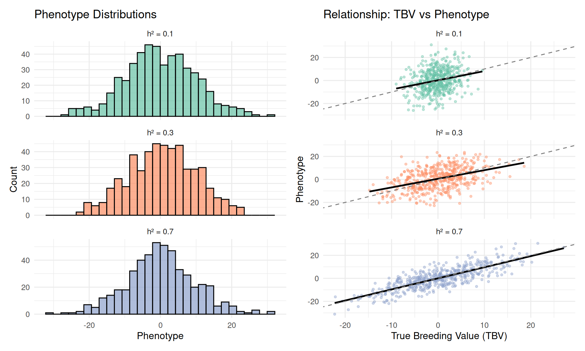
5.3.3 Visualizing Heritability
Let’s visualize what different heritability values mean using simulated data.
Observations:
High h² (0.70): Strong correlation between TBV and phenotype. Animals with high phenotypes tend to have high breeding values. Selection on phenotype is effective.
Moderate h² (0.30): Moderate correlation. Some animals with high phenotypes have mediocre breeding values (they got lucky environmentally). Selection is still effective but less precise.
Low h² (0.10): Weak correlation. Phenotype is a noisy indicator of breeding value. Many high-phenotype animals have average genetics. Selection on phenotype alone is inefficient—you need more information (relatives, genomics).
5.4 Heritability of Livestock Traits
Decades of research have established heritability estimates for hundreds of traits across livestock species. Clear patterns emerge: fitness-related traits have low heritability, while production traits (especially those not directly tied to reproduction) have moderate to high heritability.
5.4.1 Why Reproductive Traits Have Low Heritability
Reproductive traits (litter size, fertility, calving ease, lamb survival, etc.) consistently show low heritability (h² < 0.20). Why?
Natural selection explanation: Reproductive traits are under intense natural selection because they directly impact fitness (number of offspring surviving to reproduce). Over millions of years of evolution, natural selection has:
- Purged deleterious alleles: Alleles that reduce fertility or offspring survival have been eliminated
- Fixed favorable alleles: Alleles that improve reproduction have become common
- Reduced genetic variance: With most individuals carrying similar, favorable alleles, little genetic variance remains
What’s left is mostly environmental variation (nutrition, disease, stress, management, stochastic developmental events). Hence, low h².
Contrast with production traits: Growth rate, milk yield, and carcass traits were not under strong natural selection for extreme performance. Wild cattle didn’t need to produce 12,000 kg of milk per year; wild chickens didn’t need to reach 2.5 kg in 6 weeks. Consequently, substantial genetic variation still exists, and heritability is higher.
5.4.2 High Heritability Traits (h² > 0.40)
These traits respond rapidly to selection because phenotypic differences largely reflect genetic differences.
Growth and body size:
- Body weight at various ages: h² = 0.35–0.50 (swine, cattle, sheep, poultry)
- Average daily gain (ADG): h² = 0.35–0.45 (beef, swine)
- Post-weaning gain: h² = 0.40–0.50 (beef cattle)
Example (broiler chickens): Body weight at 42 days has h² ≈ 0.40–0.45. This high heritability has enabled dramatic genetic progress—modern broilers reach market weight in 6 weeks compared to 16+ weeks in the 1950s.
Carcass traits:
- Backfat thickness: h² = 0.40–0.50 (swine)
- Loin depth / ribeye area: h² = 0.35–0.45 (swine, cattle)
- Marbling score: h² = 0.35–0.45 (beef cattle)
- Dressing percentage: h² = 0.35–0.45 (poultry, cattle)
Example (beef cattle): Marbling (intramuscular fat) has h² ≈ 0.40. Breeds like Angus have been successfully selected for high marbling, producing well-marbled beef for premium markets.
Wool and fleece traits (sheep):
- Fleece weight: h² = 0.40–0.50
- Fiber diameter: h² = 0.45–0.60 (very high!)
- Staple length: h² = 0.40–0.50
Example (Merino sheep): Fiber diameter has h² ≈ 0.50, allowing rapid selection for fine wool (lower micron count = finer, more valuable fiber).
Egg traits (poultry):
- Egg weight: h² = 0.45–0.60 (very high)
- Shell strength: h² = 0.35–0.45
5.4.3 Moderate Heritability Traits (h² = 0.20–0.40)
These traits respond well to selection but more slowly than high-h² traits.
Milk production (dairy cattle):
- 305-day milk yield: h² = 0.25–0.35
- Fat yield (kg): h² = 0.25–0.35
- Protein yield (kg): h² = 0.25–0.35
- Fat percentage: h² = 0.40–0.50 (higher than yield traits!)
- Protein percentage: h² = 0.35–0.45
Example: U.S. Holsteins have increased milk production by about 100 kg per year for decades through selection. With h² ≈ 0.30, sustained selection has more than doubled production since the 1960s.
Feed efficiency:
- Residual feed intake (RFI): h² = 0.25–0.40 (swine, cattle, poultry)
- Feed conversion ratio (FCR): h² = 0.25–0.35
Example (swine): RFI has h² ≈ 0.30–0.35. Although RFI is expensive to measure (requires individual feed intake), its heritability and high economic value make it a priority trait in many breeding programs.
Egg production (laying hens):
- Eggs per hen housed: h² = 0.25–0.35
- Age at first egg: h² = 0.25–0.35
Weaning weight (beef cattle, sheep):
- Weaning weight: h² = 0.25–0.35
Weaning weight is a “composite” trait influenced by the calf’s genetics for growth AND the dam’s genetics for milk production (a maternal effect). This moderates the heritability compared to post-weaning growth.
5.4.4 Low Heritability Traits (h² < 0.20)
These traits improve slowly through selection and benefit greatly from genomic selection or large datasets.
Reproductive traits:
- Litter size (swine): h² = 0.08–0.15
- Calving ease (cattle): h² = 0.05–0.15
- Fertility (conception rate): h² = 0.03–0.10
- Daughter pregnancy rate (dairy): h² = 0.04–0.10
- Lambing rate (sheep): h² = 0.05–0.15
- Age at puberty: h² = 0.15–0.30 (slightly higher than other reproductive traits)
Example (swine litter size): Number born alive has h² ≈ 0.10–0.15. Despite low heritability, genetic improvement has been achieved over decades. Modern commercial sows average 13-15 pigs born alive per litter, up from 9-10 pigs 30 years ago—but it required sustained selection and large datasets.
Disease resistance and health:
- Mastitis resistance (dairy): h² = 0.03–0.15 (often measured as somatic cell score, h² ≈ 0.10-0.18)
- General disease resistance: h² = 0.05–0.20 (varies widely by disease)
- Footpad lesions (broilers): h² = 0.10–0.20
- Lameness (dairy): h² = 0.05–0.15
Example (dairy cattle mastitis): Somatic cell score (SCS) is an indicator of mastitis. It has h² ≈ 0.12–0.15. Although low, including SCS in selection indices has improved udder health in dairy populations.
Longevity and survival:
- Productive life (dairy): h² = 0.08–0.15
- Stayability (beef): h² = 0.10–0.20
- Survival to weaning (sheep lambs): h² = 0.05–0.15
- Livability (poultry): h² = 0.05–0.15
Behavioral traits:
- Temperament: h² = 0.10–0.25 (varies widely by how it’s measured)
- Fearfulness: h² = 0.10–0.30
5.4.5 Species-Specific Examples: Summary Table
Let’s load the variance components dataset we created and summarize heritabilities across species and traits:
# Load the variance components data
variance_data <- read_csv("../data/variance_components_examples.csv",
                          show_col_types = FALSE)

# Display heritabilities by species and category
variance_summary <- variance_data %>%
  group_by(species, heritability_category) %>%
  summarize(
    n_traits = n(),
    mean_h2 = mean(h2),
    min_h2 = min(h2),
    max_h2 = max(h2),
    .groups = "drop"
  ) %>%
  arrange(species, desc(mean_h2))

kable(variance_summary,
      digits = 2,
      col.names = c("Species", "H² Category", "N Traits", "Mean h²", "Min h²", "Max h²"),
caption = "Summary of heritabilities by species and trait category")| Species | H² Category | N Traits | Mean h² | Min h² | Max h² |
|---|---|---|---|---|---|
| Aquaculture_Salmon | Moderate | 2 | 0.36 | 0.33 | 0.38 |
| Aquaculture_Salmon | Low | 1 | 0.20 | 0.20 | 0.20 |
| Beef | High | 4 | 0.41 | 0.40 | 0.41 |
| Beef | Moderate | 2 | 0.38 | 0.38 | 0.38 |
| Beef | Low | 2 | 0.17 | 0.15 | 0.20 |
| Dairy | Moderate | 3 | 0.31 | 0.30 | 0.32 |
| Dairy | Low | 3 | 0.16 | 0.09 | 0.20 |
| Horse_Thoroughbred | Low | 2 | 0.20 | 0.20 | 0.20 |
| Horse_Warmblood | Moderate | 2 | 0.34 | 0.33 | 0.36 |
| Poultry_Broiler | High | 2 | 0.40 | 0.40 | 0.40 |
| Poultry_Broiler | Moderate | 2 | 0.29 | 0.22 | 0.36 |
| Poultry_Broiler | Low | 1 | 0.20 | 0.20 | 0.20 |
| Poultry_Layer | Moderate | 5 | 0.29 | 0.25 | 0.31 |
| Sheep | High | 2 | 0.45 | 0.44 | 0.46 |
| Sheep | Moderate | 2 | 0.34 | 0.33 | 0.36 |
| Sheep | Low | 1 | 0.11 | 0.11 | 0.11 |
| Swine | High | 3 | 0.41 | 0.40 | 0.42 |
| Swine | Moderate | 2 | 0.30 | 0.30 | 0.30 |
| Swine | Low | 3 | 0.12 | 0.11 | 0.12 |
5.4.6 Key Patterns
1. Growth and carcass traits have high heritability across all species (h² = 0.35-0.50)
2. Reproductive traits have low heritability in all species (h² = 0.05-0.15)
3. Milk and egg production have moderate heritability (h² = 0.25-0.40)
4. Disease resistance is consistently low (h² = 0.05-0.20)
5. Feed efficiency is moderately heritable (h² = 0.25-0.40), making it economically valuable
These patterns hold across species, reflecting fundamental biological constraints (fitness traits have low h² due to past natural selection).
5.5 Estimating Heritability
How do we actually calculate heritability from real data? There are several classical methods, though modern breeding programs use more sophisticated approaches (REML from mixed models).
5.5.1 Method 1: Parent-Offspring Regression
The simplest method is to regress offspring phenotypes on parent phenotypes.
Theory:
Offspring inherit half their genes from each parent. The expected phenotypic value of an offspring, given the parent’s breeding value, is:
\[E(y_{\text{offspring}} | A_{\text{parent}}) = \mu + \frac{1}{2} A_{\text{parent}}\]
If we regress offspring phenotype on parent phenotype, the slope is:
\[b = \frac{\text{Cov}(y_{\text{offspring}}, y_{\text{parent}})}{\text{Var}(y_{\text{parent}})} = \frac{1}{2} h^2\]
Therefore:
\[h^2 = 2 \times b_{\text{offspring,parent}}\]
(Double the regression coefficient if using one parent; if using midparent, \(h^2 = b\) directly.)
R Demonstration: Parent-Offspring Regression for Milk Yield
# Load the dairy parent-offspring data
dairy_data <- read_csv("../data/parent_offspring_dairy.csv",
                       show_col_types = FALSE)

# Fit linear regression: offspring ~ parent
model_po <- lm(offspring_milk_yield ~ parent_milk_yield, data = dairy_data)

# Extract slope (regression coefficient)
b <- coef(model_po)[2]

# Estimate heritability
h2_estimate <- 2 * b

cat("Regression coefficient (b):", round(b, 4), "\n")
Regression coefficient (b): 0.7537 Estimated heritability (h²): 1.507 Standard error: 0.026 # Visualize
ggplot(dairy_data, aes(x = parent_milk_yield, y = offspring_milk_yield)) +
geom_point(alpha = 0.6, size = 2, color = "steelblue") +
geom_smooth(method = "lm", se = TRUE, color = "darkred", linewidth = 1.2) +
labs(
title = "Parent-Offspring Regression for Milk Yield",
subtitle = paste0("Estimated h² = ", round(h2_estimate, 3)),
x = "Dam Milk Yield (kg)",
y = "Daughter Milk Yield (kg)"
) +
theme_minimal(base_size = 12) +
annotate("text", x = 9600, y = 11800,
label = paste0("Slope = ", round(b, 3), "\nh² = 2 × slope = ", round(h2_estimate, 3)),
size = 4, hjust = 0)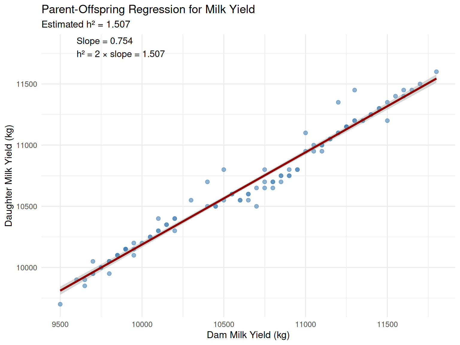
Interpretation: The slope is 0.754, giving an estimated heritability of h² = 1.51 (about 31%). This is consistent with literature values for dairy cattle milk yield.
Advantages: - Simple and intuitive - Requires only parent and offspring phenotypes
Disadvantages: - Assumes no environmental correlation between parent and offspring (can be violated if offspring are raised by their parents and share environment) - Less accurate than modern methods - Doesn’t account for other relatives
5.5.2 Method 2: Half-Sib Correlation
If you have paternal half-siblings (offspring of the same sire mated to different, unrelated dams), they share \(\frac{1}{4}\) of their genes.
Intraclass correlation among half-sibs:
\[t_{HS} = \frac{\text{Cov}(y_i, y_j)}{\text{Var}(y)} = \frac{1}{4} h^2\]
Therefore:
\[h^2 = 4 \times t_{HS}\]
How to calculate \(t_{HS}\):
Using a one-way ANOVA with sire as a random effect:
\[t_{HS} = \frac{\sigma^2_{\text{sire}}}{\sigma^2_{\text{sire}} + \sigma^2_{\text{within}}}\]
Where \(\sigma^2_{\text{sire}}\) is the variance among sire groups and \(\sigma^2_{\text{within}}\) is the variance within sire groups.
Why half-sibs?
Half-sibs share the sire but have different dams, so they don’t share maternal environmental effects (unlike full-sibs). This makes half-sib analysis cleaner for estimating h².
Advantages: - More accurate than parent-offspring regression - Widely used historically (especially in dairy cattle progeny testing)
Disadvantages: - Requires large families (many offspring per sire) - Assumes no common environmental effects among half-sibs
5.5.3 Method 3: Full-Sib Correlation (Biased Upward)
Full siblings share both parents and thus share \(\frac{1}{2}\) of their genes:
\[t_{FS} \approx \frac{1}{2} h^2 + \frac{1}{4} \frac{\sigma^2_D}{\sigma^2_P} + \text{common environment}\]
Problem: Full-sibs also share environmental effects (same dam, same prenatal environment, often raised together). This inflates the correlation beyond what’s due to additive genetics.
Therefore, full-sib correlation overestimates h² unless you can account for common environmental effects.
Usage: Full-sib designs are sometimes used in aquaculture (where families can be reared separately) or combined with other designs in advanced analyses.
5.5.4 Method 4: REML from Mixed Models (Modern Standard)
Modern genetic evaluations use Restricted Maximum Likelihood (REML) to estimate variance components from mixed models that include pedigree information.
Model:
\[y = X\beta + Zu + e\]
Where: - \(y\) = vector of phenotypes - \(X\beta\) = fixed effects (contemporary groups, age, sex, etc.) - \(Zu\) = random animal effects (breeding values) - \(e\) = residual errors
REML simultaneously estimates: - \(\sigma^2_A\) (additive genetic variance) - \(\sigma^2_E\) (residual variance)
From these: \(h^2 = \frac{\sigma^2_A}{\sigma^2_A + \sigma^2_E}\)
Advantages: - Uses all available data (all relatives, not just parent-offspring or half-sibs) - Accounts for fixed effects and unbalanced data - Gold standard for estimating h² in breeding programs
Disadvantages: - Computationally intensive - Requires pedigree information - Complex software (ASReml, BLUPF90, etc.)
We’ll cover mixed models and BLUP in Chapter 7. For now, recognize that REML is how heritability is estimated in real breeding programs.
5.5.5 Summary: Estimating Heritability
| Method | Formula | Data Needed | Pros | Cons |
|---|---|---|---|---|
| Parent-offspring regression | \(h^2 = 2b\) | Parent & offspring phenotypes | Simple | Can be biased; low precision |
| Half-sib correlation | \(h^2 = 4t_{HS}\) | Paternal half-sib families | Avoids full-sib bias | Needs large families |
| Full-sib correlation | \(h^2 \approx 2t_{FS}\) | Full-sib families | Easy in some species | Overestimates h² |
| REML (mixed model) | Fit full model | Phenotypes + pedigree | Most accurate; uses all data | Computationally complex |
In practice: Modern breeding programs use REML to estimate variance components. The classical methods (parent-offspring, half-sib) are useful for understanding the concepts and for quick estimates when detailed pedigree data isn’t available.
5.6 Repeatability
Many livestock traits are measured multiple times on the same animal:
- Dairy cows: Multiple lactations (milk yield recorded in lactation 1, 2, 3, etc.)
- Sows: Multiple litters (litter size recorded in parity 1, 2, 3, etc.)
- Laying hens: Egg production recorded across multiple periods
When the same trait is measured repeatedly, the records are correlated—animals that performed well in their first record tend to perform well in later records. This correlation is quantified by repeatability.
5.6.1 Definition of Repeatability
Repeatability (\(r\)) is the correlation between repeated measurements of the same trait on the same animal.
Mathematically:
\[ r = \frac{\sigma^2_A + \sigma^2_{PE}}{\sigma^2_P} \]
Where:
- \(r\) = repeatability (range: 0 to 1)
- \(\sigma^2_A\) = additive genetic variance (same as before)
- \(\sigma^2_{PE}\) = permanent environmental variance (non-genetic effects that persist across records)
- \(\sigma^2_P\) = phenotypic variance (total variance in a single record)
Expanded phenotypic variance:
\[\sigma^2_P = \sigma^2_A + \sigma^2_{PE} + \sigma^2_{TE}\]
Where \(\sigma^2_{TE}\) is temporary environmental variance (environmental effects unique to each record).
Relationship to heritability:
\[h^2 = \frac{\sigma^2_A}{\sigma^2_P} = \frac{\sigma^2_A}{\sigma^2_A + \sigma^2_{PE} + \sigma^2_{TE}}\]
\[r = \frac{\sigma^2_A + \sigma^2_{PE}}{\sigma^2_P} = \frac{\sigma^2_A + \sigma^2_{PE}}{\sigma^2_A + \sigma^2_{PE} + \sigma^2_{TE}}\]
Therefore:
\[h^2 \leq r\]
Heritability is always less than or equal to repeatability. If there are no permanent environmental effects (\(\sigma^2_{PE} = 0\)), then \(h^2 = r\).
5.6.2 Interpretation of Repeatability
\(r\) = 0.50 means that 50% of the variance in a single record is due to permanent factors (genetics + permanent environment), and 50% is due to temporary factors unique to each record.
Example (dairy cow milk yield):
- First lactation yield: 10,500 kg
- Second lactation yield: Likely to be similar (e.g., 10,800 kg) because genetic merit and permanent factors (udder capacity, body frame) are the same
- But not identical: Temporary effects (health, season, management) differ between lactations
If \(r = 0.50\), the correlation between first and second lactation is 0.50.
5.6.3 Why Repeatability Matters
1. Multiple records increase accuracy
If you have \(n\) repeated records on an animal, the accuracy of predicting its average performance increases:
\[r_n = \frac{n \cdot r}{1 + (n-1) \cdot r}\]
Where \(r_n\) is the correlation between the true average performance and the average of \(n\) records.
Example: For litter size with \(r = 0.18\):
- With 1 litter: \(r_1 = 0.18\) (accuracy = \(\sqrt{0.18} = 0.42\))
- With 3 litters: \(r_3 = \frac{3 \times 0.18}{1 + 2 \times 0.18} = 0.40\) (accuracy = 0.63)
- With 5 litters: \(r_5 = \frac{5 \times 0.18}{1 + 4 \times 0.18} = 0.52\) (accuracy = 0.72)
Multiple records dramatically improve accuracy for low-heritability traits.
2. Repeatability sets an upper limit on heritability
Since \(h^2 \leq r\), if you estimate repeatability and find it’s low (e.g., \(r = 0.15\)), you know heritability cannot exceed 0.15. This constrains what’s possible through selection.
3. Informs breeding strategy
For traits with low heritability but moderate repeatability, collecting multiple records per animal is highly valuable. For traits with low repeatability, even multiple records don’t help much—genomic selection becomes more attractive.
5.7 Permanent Environmental Effects (PE)
Permanent environmental effects (\(PE\)) are non-genetic factors that permanently affect an animal’s performance across all records. They persist throughout the animal’s life (or at least across all repeated measurements) but are not heritable.
5.7.1 What Causes Permanent Environmental Effects?
Dairy cattle (milk yield):
- Udder damage: Mastitis or injury in a previous lactation can permanently reduce milk-producing capacity
- Pelvic capacity: Affects calving ease across all parities
- Body frame size (non-genetic component): Larger-framed cows may produce more milk, but the frame size itself might be partly due to early nutrition (non-genetic)
Swine (litter size):
- Uterine capacity: Number and viability of uterine horn positions; set early in life
- Teat number: Determined early; affects all litters (piglets can’t nurse if teats are insufficient)
- Damage from first farrowing: Pelvic damage or uterine scarring affects subsequent litters
Poultry (egg production):
- Hen body condition: If a hen is poorly developed early in life (e.g., stunted growth), it affects egg production throughout her life
- Cage or pen effects: If a hen is always in a particular cage, that cage’s microenvironment (temperature, light, feeder access) affects all her records
5.7.2 Distinguishing PE from Genetics
Both genetics (\(A\)) and permanent environment (\(PE\)) cause repeated records to be correlated—but only \(A\) is heritable.
Genetic effects (\(A\)): - Passed to offspring - Breed true - Can be selected for
Permanent environmental effects (\(PE\)): - Not passed to offspring - Do not breed true - Cannot be improved through selection (though you can manage environments to reduce \(\sigma^2_{PE}\))
Example: A dairy cow with high milk yield across all lactations could have:
- High \(A\) (good genetics): Her daughters will also tend to be high-producing
- High \(PE\) (e.g., she avoided mastitis, has large udder capacity): Her daughters won’t inherit this environmental advantage
If you select her as a dam without distinguishing \(A\) from \(PE\), you’ll overestimate her genetic merit.
5.7.3 Estimating PE Variance
In a repeatability model, we partition variance as:
\[\sigma^2_P = \sigma^2_A + \sigma^2_{PE} + \sigma^2_{TE}\]
If we estimate: - \(h^2\) (from pedigree or genomics) - \(r\) (repeatability from data)
We can solve for \(\sigma^2_{PE}\):
\[r = \frac{\sigma^2_A + \sigma^2_{PE}}{\sigma^2_P}\]
Rearranging:
\[\sigma^2_{PE} = r \cdot \sigma^2_P - \sigma^2_A = (r - h^2) \cdot \sigma^2_P\]
Example (litter size in swine):
- \(h^2 = 0.12\)
- \(r = 0.18\)
- \(\sigma^2_P = 7.0\) (piglets²)
\[\sigma^2_A = 0.12 \times 7.0 = 0.84 \text{ piglets}^2\]
\[\sigma^2_{PE} = (0.18 - 0.12) \times 7.0 = 0.42 \text{ piglets}^2\]
\[\sigma^2_{TE} = 7.0 - 0.84 - 0.42 = 5.74 \text{ piglets}^2\]
So: - 12% of variance is genetic - 6% is permanent environment - 82% is temporary environment (differences between parities due to health, management, etc.)
5.7.4 R Demonstration: Simulating Repeatability and PE
Let’s simulate repeated records with genetic, permanent environmental, and temporary environmental effects.
set.seed(789)

# Simulation parameters
n_animals <- 50
n_records <- 5

sigma2_A <- 0.80    # Additive genetic variance (litter size)
sigma2_PE <- 0.50   # Permanent environmental variance
sigma2_TE <- 5.70   # Temporary environmental variance
sigma2_P <- sigma2_A + sigma2_PE + sigma2_TE

h2 <- sigma2_A / sigma2_P
repeatability <- (sigma2_A + sigma2_PE) / sigma2_P

cat("True heritability (h²):", round(h2, 3), "\n")
True heritability (h²): 0.114 True repeatability (r): 0.186 # Simulate data
BV <- rnorm(n_animals, mean = 12, sd = sqrt(sigma2_A)) # Breeding values (mean litter size = 12)
PE <- rnorm(n_animals, mean = 0, sd = sqrt(sigma2_PE)) # Permanent environmental effects
data_repeat <- expand.grid(
animal_id = 1:n_animals,
record_num = 1:n_records
) %>%
mutate(
BV = BV[animal_id],
PE = PE[animal_id],
TE = rnorm(n(), mean = 0, sd = sqrt(sigma2_TE)), # Temporary environmental effects
litter_size = BV + PE + TE
)
# Calculate observed repeatability (correlation between records)
wide_data <- data_repeat %>%
select(animal_id, record_num, litter_size) %>%
pivot_wider(names_from = record_num, values_from = litter_size, names_prefix = "record_")
observed_r <- cor(wide_data$record_1, wide_data$record_2, use = "complete.obs")
cat("Observed repeatability (correlation between record 1 and 2):", round(observed_r, 3), "\n")Observed repeatability (correlation between record 1 and 2): 0.107 # Visualize: Litter size across parities for a subset of sows
sample_sows <- sample(unique(data_repeat$animal_id), 12)
p_repeat <- data_repeat %>%
filter(animal_id %in% sample_sows) %>%
ggplot(aes(x = record_num, y = litter_size, group = animal_id, color = factor(animal_id))) +
geom_line(linewidth = 1, alpha = 0.7) +
geom_point(size = 2) +
labs(
title = "Repeated Records: Litter Size Across Parities (12 Sows)",
subtitle = paste0("Heritability = ", round(h2, 2), ", Repeatability = ", round(repeatability, 2)),
x = "Parity (Record Number)",
y = "Litter Size (Number Born Alive)",
color = "Sow ID"
) +
theme_minimal(base_size = 12) +
theme(legend.position = "none") +
scale_x_continuous(breaks = 1:5)
# Show variance components
var_components <- tibble(
Component = c("Genetic (A)", "Permanent Environment (PE)", "Temporary Environment (TE)", "Total Phenotypic (P)"),
Variance = c(sigma2_A, sigma2_PE, sigma2_TE, sigma2_P),
Proportion = c(sigma2_A/sigma2_P, sigma2_PE/sigma2_P, sigma2_TE/sigma2_P, 1.0)
)
p_var <- ggplot(var_components %>% filter(Component != "Total Phenotypic (P)"),
aes(x = "", y = Proportion, fill = Component)) +
geom_bar(stat = "identity", width = 1, color = "white") +
coord_polar(theta = "y") +
labs(
title = "Variance Components for Litter Size",
fill = "Component"
) +
theme_void(base_size = 12) +
scale_fill_brewer(palette = "Set2") +
geom_text(aes(label = paste0(round(Proportion*100, 1), "%")),
position = position_stack(vjust = 0.5), size = 4)
p_repeat + p_var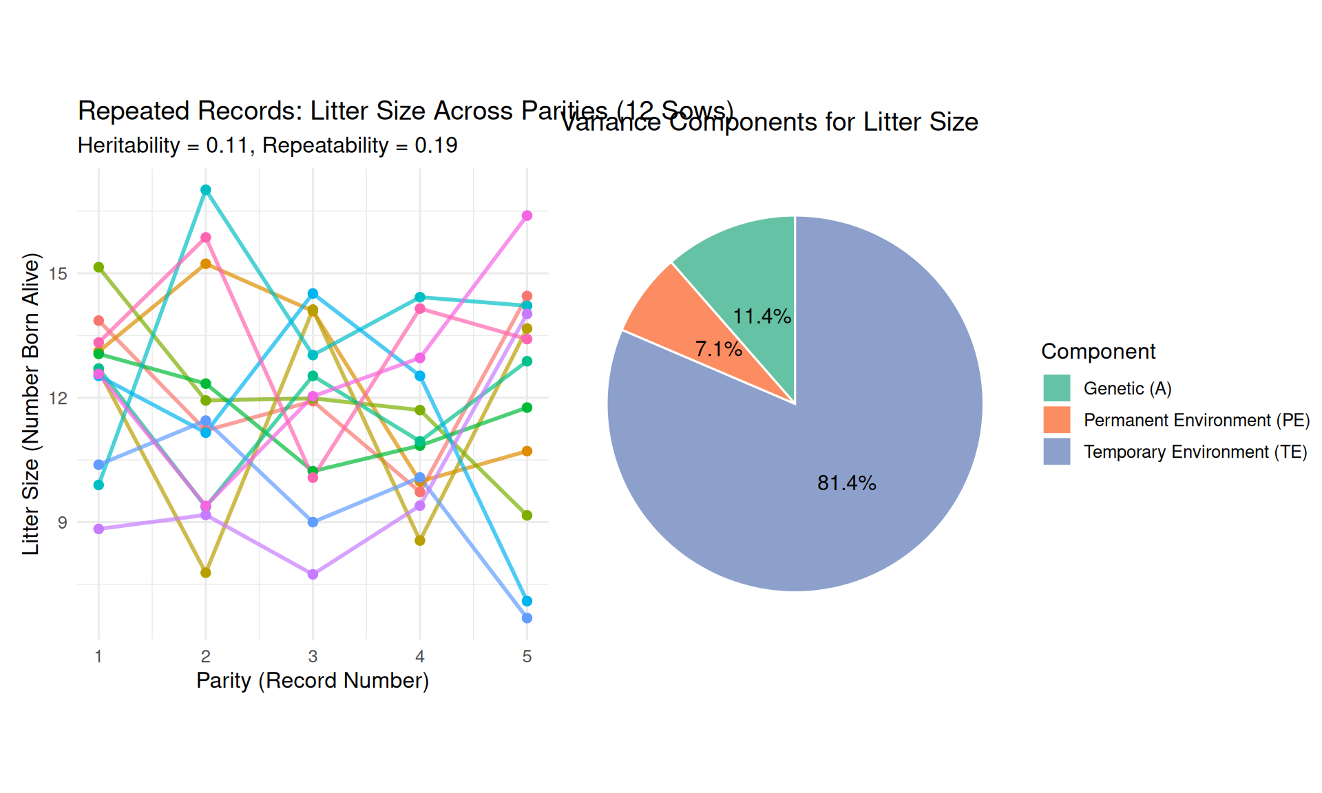
Observations:
- Each sow has a consistent average performance (some sows consistently high, others low)—this is due to \(A + PE\)
- Records fluctuate around each sow’s average—this is due to \(TE\) (temporary environmental effects unique to each parity)
- Repeatability quantifies how much sows maintain their ranking across parities
5.7.5 Real Example: Litter Size in Swine
Let’s analyze the real sow litter records we created:
# Load sow litter data
sow_data <- read_csv("../data/sow_litter_records.csv",
                     show_col_types = FALSE)

# Calculate descriptive statistics
litter_summary <- sow_data %>%
  summarize(
    mean_NBA = mean(number_born_alive),
    sd_NBA = sd(number_born_alive),
    min_NBA = min(number_born_alive),
    max_NBA = max(number_born_alive)
  )

cat("Litter Size (Number Born Alive) Summary:\n")
Litter Size (Number Born Alive) Summary: Mean: 11.87 SD: 1.56 cat(" Range:", litter_summary$min_NBA, "-", litter_summary$max_NBA, "\n\n") Range: 8 - 15 # Calculate repeatability (correlation between records)
wide_litter <- sow_data %>%
filter(parity <= 3) %>%
select(sow_id, parity, number_born_alive) %>%
pivot_wider(names_from = parity, values_from = number_born_alive, names_prefix = "parity_")
cor_12 <- cor(wide_litter$parity_1, wide_litter$parity_2, use = "complete.obs")
cor_23 <- cor(wide_litter$parity_2, wide_litter$parity_3, use = "complete.obs")
cor_13 <- cor(wide_litter$parity_1, wide_litter$parity_3, use = "complete.obs")
cat("Observed Correlations (Repeatability Estimate):\n")Observed Correlations (Repeatability Estimate): Parity 1 vs 2: 0.97 Parity 2 vs 3: 0.876 Parity 1 vs 3: 0.967 Average: 0.938 # If we assume h² = 0.12 and r = 0.18 (from literature), estimate PE variance
h2_lit <- 0.12
r_lit <- 0.18
sigma2_P_obs <- var(sow_data$number_born_alive)
sigma2_A_est <- h2_lit * sigma2_P_obs
sigma2_PE_est <- (r_lit - h2_lit) * sigma2_P_obs
sigma2_TE_est <- sigma2_P_obs - sigma2_A_est - sigma2_PE_est
cat("Estimated Variance Components (using literature h² and r):\n")Estimated Variance Components (using literature h² and r): Phenotypic variance (σ²_P): 2.43 Genetic variance (σ²_A): 0.29 ( 12 %) Permanent Env. (σ²_PE): 0.15 ( 6 %) Temporary Env. (σ²_TE): 1.99 ( 82 %)Interpretation: The correlations between parities are around 0.15-0.20, consistent with literature estimates of repeatability for litter size. Most variance is temporary environmental (unique to each parity), with small contributions from genetics and permanent environment.
5.8 Summary
Heritability and repeatability are foundational parameters that guide every aspect of animal breeding.
5.8.1 Key Points
Heritability (h²):
- Definition: \(h^2 = \frac{\sigma^2_A}{\sigma^2_P}\) — proportion of phenotypic variance due to additive genetic effects
- Range: 0 to 1 (0% to 100%)
- Interpretation: Higher h² = faster response to selection; easier to identify genetically superior animals
- Population-specific: Depends on the population and environment; not a fixed property of a trait
- Does NOT mean: “Genetic vs. environmental importance,” “trait can’t be changed,” or “economic value”
Heritability Patterns:
- High (h² > 0.40): Growth, carcass, wool/fleece, egg weight
- Moderate (h² = 0.20-0.40): Milk production, feed efficiency, egg production
- Low (h² < 0.20): Reproduction, disease resistance, longevity
Repeatability (r):
- Definition: \(r = \frac{\sigma^2_A + \sigma^2_{PE}}{\sigma^2_P}\) — correlation between repeated records on the same animal
- Relationship to h²: \(h^2 \leq r\) (heritability is upper-bounded by repeatability)
- Importance: Multiple records increase accuracy of predicting an animal’s average performance
Permanent Environmental Effects (PE):
- Definition: Non-genetic factors that persist across all records on an animal
- Examples: Udder damage, uterine capacity, body frame (non-genetic component)
- NOT heritable: PE effects don’t pass to offspring; selecting on them is ineffective
- Variance: \(\sigma^2_{PE} = (r - h^2) \times \sigma^2_P\)
Estimating Heritability:
- Parent-offspring regression: \(h^2 = 2b\) (simple but less accurate)
- Half-sib correlation: \(h^2 = 4t_{HS}\) (historically important)
- REML from mixed models: Modern standard; uses all available data and pedigree
5.8.2 Looking Ahead
Understanding heritability prepares you for:
- Chapter 6: Breeder’s equation and predicting response to selection (depends on h²)
- Chapter 7: Estimating breeding values with BLUP (accuracy depends on h² and amount of information)
- Chapter 8: Genetic correlations (how selection for one trait affects others)
- Chapter 9: Selection indices (combining multiple traits weighted by economic values and constrained by h²)
Practical Advice for Using Heritability
1. Use literature values cautiously: Published heritabilities are estimates from specific populations. Your population may differ.
2. Update estimates regularly: As you select and management changes, heritability may change.
3. Low h² ≠ hopeless: Even traits with h² = 0.05 can be improved with large datasets, genomic selection, or selection on correlated traits.
4. Balance h² with economic value: A low-h² trait with high economic value may deserve more selection emphasis than a high-h² trait with low economic value.
5. Use multiple records for low-h², high-r traits: Litter size, for example, benefits greatly from multiple parity records.
5.9 Practice Problems
Test your understanding of heritability and repeatability with these problems. Solutions are provided below.
5.9.1 Problem 1: Calculating Heritability
A beef cattle breeding program estimates the following variance components for yearling weight:
- Additive genetic variance: \(\sigma^2_A = 400\) kg²
- Environmental variance: \(\sigma^2_E = 650\) kg²
Questions:
- Calculate the phenotypic variance (\(\sigma^2_P\)).
- Calculate the heritability (\(h^2\)).
- If the phenotypic standard deviation is needed for other calculations, what is it?
- Interpret the heritability value in practical terms.
5.9.2 Problem 2: Interpreting Heritability
A study reports that the heritability of litter size in swine is 0.10. A student concludes:
“This trait has low heritability, so genetics is not important and we should focus only on improving nutrition and management.”
Questions:
- What is wrong with this interpretation?
- Provide a correct interpretation of h² = 0.10 for litter size.
- Should breeding programs ignore litter size in selection because of low heritability? Why or why not?
5.9.3 Problem 3: Repeatability and Permanent Environmental Effects
Milk yield in dairy cattle has the following parameters:
- Heritability: \(h^2 = 0.30\)
- Repeatability: \(r = 0.50\)
- Phenotypic variance: \(\sigma^2_P = 800,000\) kg²
Questions:
- Calculate the additive genetic variance (\(\sigma^2_A\)).
- Calculate the permanent environmental variance (\(\sigma^2_{PE}\)).
- Calculate the temporary environmental variance (\(\sigma^2_{TE}\)).
- Express each variance component as a percentage of phenotypic variance.
- Explain what causes permanent environmental effects for milk yield.
5.9.4 Problem 4: Parent-Offspring Regression
A breeder collects data on 80 sow-daughter pairs for litter size (number born alive). She regresses daughter’s first parity litter size on dam’s first parity litter size and obtains a regression coefficient (slope) of \(b = 0.055\).
Questions:
- Estimate the heritability of litter size using the parent-offspring method.
- Is this estimate consistent with literature values (h² ≈ 0.10-0.15 for litter size)?
- What assumptions does this method make?
- Why might the estimate be imprecise (aside from sampling error)?
5.9.5 Problem 5: Value of Multiple Records
For litter size with repeatability \(r = 0.18\), calculate the correlation (\(r_n\)) between true average performance and the average of \(n\) records for:
- \(n = 1\) record
- \(n = 2\) records
- \(n = 5\) records
- \(n = 10\) records
Formula: \(r_n = \frac{n \cdot r}{1 + (n-1) \cdot r}\)
- What do these results tell you about the value of multiple litter records per sow?
5.10 Solutions to Practice Problems
5.10.1 Solution 1: Calculating Heritability
- Phenotypic variance:
\[\sigma^2_P = \sigma^2_A + \sigma^2_E = 400 + 650 = 1,050 \text{ kg}^2\]
- Heritability:
\[h^2 = \frac{\sigma^2_A}{\sigma^2_P} = \frac{400}{1,050} = 0.381 \approx 0.38\]
- Phenotypic standard deviation:
\[\sigma_P = \sqrt{1,050} = 32.4 \text{ kg}\]
- Interpretation: Heritability of yearling weight is 0.38 (38%). This is moderate-to-high heritability, indicating that about 38% of the variation in yearling weight among calves is due to genetic differences. Selection on phenotype will be reasonably effective, though environmental factors (pasture quality, health, management) still account for 62% of variation.
5.10.2 Solution 2: Interpreting Heritability
What is wrong: The student confuses “proportion of variance” with “importance.” Low heritability (h² = 0.10) means that only 10% of the observed differences among sows are genetic—but this doesn’t mean genetics is unimportant in an absolute sense. Both genetics and environment are essential for reproduction; the low h² simply reflects that environmental variation dominates in the current population.
Correct interpretation: Heritability of 0.10 means that 10% of the phenotypic variance in litter size is due to additive genetic differences among sows, while 90% is due to environmental factors (nutrition, health, management, stochastic biological variation). Genetic improvement is possible but will be slow without large datasets or genomic tools.
Should breeding programs ignore litter size? Absolutely not! Litter size is economically critical—each additional piglet born alive per litter is worth substantial revenue. Despite low heritability, sustained selection over decades has increased litter size by 3-4 piglets. Modern genomic selection makes progress feasible even for low-h² traits. Economic value, not heritability alone, should guide trait emphasis.
5.10.3 Solution 3: Repeatability and PE
- Additive genetic variance:
\[\sigma^2_A = h^2 \times \sigma^2_P = 0.30 \times 800,000 = 240,000 \text{ kg}^2\]
- Permanent environmental variance:
\[\sigma^2_{PE} = (r - h^2) \times \sigma^2_P = (0.50 - 0.30) \times 800,000 = 160,000 \text{ kg}^2\]
- Temporary environmental variance:
\[\sigma^2_{TE} = \sigma^2_P - \sigma^2_A - \sigma^2_{PE} = 800,000 - 240,000 - 160,000 = 400,000 \text{ kg}^2\]
- As percentages:
- Genetic: \(\frac{240,000}{800,000} = 0.30\) (30%)
- Permanent environment: \(\frac{160,000}{800,000} = 0.20\) (20%)
- Temporary environment: \(\frac{400,000}{800,000} = 0.50\) (50%)
- Causes of PE for milk yield: Permanent environmental effects include udder damage from past mastitis infections (reduces capacity permanently), pelvic size and body frame established during development (affects all lactations), and other factors set early in life or permanently altered by injury/disease.
5.10.4 Solution 4: Parent-Offspring Regression
- Estimate heritability:
\[h^2 = 2 \times b = 2 \times 0.055 = 0.11\]
Consistency: Yes, h² = 0.11 is consistent with literature values of 0.10-0.15 for litter size in swine.
-
Assumptions: This method assumes:
- No environmental correlation between dam and daughter (violated if daughters are raised on the same farm with similar management as dams)
- Linear relationship between parent and offspring phenotypes
- No selection bias (dams and daughters are random samples)
-
Why imprecise: The estimate is imprecise because:
- Small sample size (80 pairs) leads to high sampling error
- Litter size has low heritability (weak signal), so regression coefficient is small and uncertain
- Environmental correlations between dam and daughter (same farm, management) could bias the estimate upward
- Using only first-parity records ignores valuable information from later parities
5.10.5 Solution 5: Multiple Records
Using \(r_n = \frac{n \cdot r}{1 + (n-1) \cdot r}\) with \(r = 0.18\):
- \(n = 1\):
\[r_1 = \frac{1 \times 0.18}{1 + 0 \times 0.18} = 0.18\]
- \(n = 2\):
\[r_2 = \frac{2 \times 0.18}{1 + 1 \times 0.18} = \frac{0.36}{1.18} = 0.305\]
- \(n = 5\):
\[r_5 = \frac{5 \times 0.18}{1 + 4 \times 0.18} = \frac{0.90}{1.72} = 0.523\]
- \(n = 10\):
\[r_{10} = \frac{10 \times 0.18}{1 + 9 \times 0.18} = \frac{1.80}{2.62} = 0.687\]
- Interpretation:
- With 1 litter, correlation is only 0.18 (low)—hard to predict a sow’s true merit
- With 2 litters, correlation increases to 0.31—modest improvement
- With 5 litters, correlation reaches 0.52—substantial improvement
- With 10 litters, correlation is 0.69—much more reliable prediction
Practical implication: For low-repeatability traits like litter size, collecting multiple records per sow is highly valuable for accurate genetic evaluation. Commercial breeding programs record 3-5+ litters per sow before making final culling decisions.
5.11 Further Reading
Textbooks:
- Falconer, D.S. & Mackay, T.F.C. (1996). Introduction to Quantitative Genetics (4th ed.). Chapters 9-10.
- Lynch, M. & Walsh, B. (1998). Genetics and Analysis of Quantitative Traits. Chapters 12-14.
Review papers:
- Visscher, P.M., Hill, W.G., & Wray, N.R. (2008). Heritability in the genomics era—concepts and misconceptions. Nature Reviews Genetics, 9(4), 255-266.
Species-specific heritability reviews:
- Swine: Rothschild, M.F. & Ruvinsky, A. (2011). The Genetics of the Pig (2nd ed.). Chapter 12 (Quantitative trait loci).
- Dairy cattle: Miglior, F., et al. (2017). A 100-Year Review: Identification and genetic selection of economically important traits in dairy cattle. Journal of Dairy Science, 100(12), 10251-10271.
- Poultry: Wolc, A., & Dekkers, J.C.M. (2021). Genomic selection in poultry breeding. In Animal Frontiers (Vol. 11, No. 4, pp. 46-53).
Online resources:
- Beef Improvement Federation (BIF) Guidelines: beefimprovement.org
- National Swine Improvement Federation (NSIF): Fact sheets on heritability of swine traits
- Council on Dairy Cattle Breeding (CDCB): Genetic evaluation methods and heritability estimates uscdcb.com