| Proportion Selected (p) | Selection Intensity (i) | Description |
|---|---|---|
| 0.01 (1%) | 2.67 | Extremely intense |
| 0.02 (2%) | 2.42 | Very intense |
| 0.05 (5%) | 2.06 | High intensity |
| 0.10 (10%) | 1.76 | Moderate-high intensity |
| 0.20 (20%) | 1.40 | Moderate intensity |
| 0.30 (30%) | 1.16 | Moderate-low intensity |
| 0.40 (40%) | 0.97 | Low intensity |
| 0.50 (50%) | 0.80 | Very low intensity |
6 The Breeder’s Equation and Selection Response
Learning Objectives
By the end of this chapter, you will be able to:
- State and apply the breeder’s equation
- Explain how each of the four factors influences response to selection
- Describe trade-offs between accuracy, intensity, and generation interval
- Compare different selection strategies using the breeder’s equation
- Calculate expected response to selection for livestock traits
- Understand how genomic selection revolutionized animal breeding
6.1 Introduction
Imagine you’re the director of genetics for a major swine breeding company. Your company has invested millions in collecting phenotypic data on growth rate, feed efficiency, and meat quality across thousands of pigs. You have genomic data on all breeding candidates. Now you face a critical decision: Should you select replacement boars at 6 months of age using genomic predictions, or wait until 12 months when you have their own feed efficiency records? Both strategies have advantages—genomic selection is faster but less accurate, while waiting for performance data is more accurate but delays selection by six months.
This type of trade-off is at the heart of every breeding program. The breeder’s equation provides a mathematical framework for making these decisions. It shows us exactly how four factors—selection intensity, accuracy, genetic variation, and generation interval—combine to determine the rate of genetic improvement. Understanding this equation and the trade-offs among these factors is fundamental to designing effective breeding programs.
The breeder’s equation might seem deceptively simple at first glance, but its implications are profound. It explains why poultry breeding programs achieve genetic gains 10 times faster than beef cattle programs. It tells us why genomic selection roughly doubled the rate of genetic gain in dairy cattle since 2009. And it guides decisions about how to allocate limited resources across traits, sexes, and selection pathways.
In this chapter, we’ll build intuition for each component of the breeder’s equation before diving into the mathematics. We’ll work through numerous examples across livestock species, comparing different selection strategies and understanding trade-offs. By the end, you’ll be equipped to predict selection response, compare breeding strategies, and optimize breeding programs for maximum genetic gain.
6.2 The Breeder’s Equation
6.2.1 The Fundamental Equation
The breeder’s equation, also called the key equation in animal breeding, predicts how much genetic progress we can achieve per unit time:
\[ R = \frac{i \times r \times \sigma_A}{L} \]
Where:
- R = response to selection per year (or per generation if L = 1)
- i = selection intensity (standardized selection differential)
- r = accuracy of selection (correlation between EBV and TBV)
- σA = additive genetic standard deviation
- L = generation interval (average age of parents when offspring are born)
This equation is sometimes written as R = i × r × σA / L or equivalently as R per generation = i × r × σA when we’re thinking about response per generation rather than per year.
6.2.2 Understanding the Equation Intuitively
Before we dive into the mathematics, let’s build intuition for what each factor means:
Selection intensity (i): How hard are we selecting? If we choose only the top 1% of animals as parents, we’re selecting more intensely than if we choose the top 50%. Higher intensity means we’re keeping animals with higher breeding values, leading to more genetic progress.
Accuracy (r): How well can we predict which animals are genetically superior? If we have lots of information (genomic data, progeny records, relatives’ performance), we can rank animals more accurately. Better accuracy means we’re more likely to select the truly superior animals.
Genetic standard deviation (σA): How much genetic variation exists in the population? Some traits and populations have more genetic variation than others. More variation means there’s more potential for improvement through selection.
Generation interval (L): How quickly do we cycle through generations? Poultry can produce offspring at one year of age, while horses might not breed until 5+ years old. Shorter generation intervals mean we can accumulate genetic gains faster.
6.2.3 Why the Four Factors Multiply
Notice that the four factors multiply together (with L in the denominator). This has important implications:
- Improving any factor increases response: If we double accuracy, we double the response to selection (assuming other factors stay constant).
- Zero in any factor means zero progress: If accuracy is zero (random selection), or if there’s no genetic variation (σA = 0), we make no genetic progress regardless of the other factors.
- Trade-offs matter: Because factors multiply, a small improvement in one factor can sometimes give more progress than a large improvement in another factor.
The division by generation interval (L) is critical—it converts response per generation into response per year. A breeding program might achieve great response per generation, but if generations take 8 years, the annual progress will be slow.
Historical Context
The breeder’s equation was formalized by Jay Lush in the 1930s-1940s, building on earlier work by R.A. Fisher and Sewall Wright. Lush, often called the “father of modern animal breeding,” recognized that genetic progress depends on these four factors. His insights transformed animal breeding from an art into a science. The equation remains the foundation of all modern breeding programs, from dairy cattle to poultry to aquaculture.
6.2.4 A Simple Example
Let’s see the equation in action with a simple example. Suppose we’re selecting for increased body weight in broiler chickens:
- i = 2.06 (selecting the top 5% of males and females)
- r = 0.65 (using genomic selection on young birds)
- σA = √18,000 = 134.2 grams (the standard deviation of breeding values)
- L = 1.0 year (chickens mature quickly)
Expected annual response:
\[ R = \frac{2.06 \times 0.65 \times 134.2}{1.0} = 180 \text{ grams per year} \]
This means we expect the average body weight of broiler chickens to increase by about 180 grams every year due to selection. Over 10 years, that’s 1,800 grams (1.8 kg) of genetic improvement—a substantial change!
Now let’s compare this to beef cattle selecting for weaning weight:
- i = 1.76 (selecting the top 10% due to lower reproductive rates)
- r = 0.60 (using genomic EPDs)
- σA = √180 = 13.4 kg
- L = 5.0 years (cattle take longer to mature and reproduce)
Expected annual response:
\[ R = \frac{1.76 \times 0.60 \times 13.4}{5.0} = 2.8 \text{ kg per year} \]
Notice that even though we have similar intensity, accuracy, and genetic variation (relative to trait scale), the beef cattle program achieves much slower annual progress due to the longer generation interval. This example illustrates why generation interval is such a critical factor in determining breeding program success.
6.3 Selection Intensity (i)
6.3.1 What Is Selection Intensity?
Selection intensity measures how hard we’re selecting—how restrictive we are in choosing parents. When we select only the very best animals, we’re applying high selection intensity. When we’re less restrictive, intensity is lower.
Formally, selection intensity is the standardized selection differential:
\[ i = \frac{S}{\sigma_P} \]
Where: - S = selection differential (mean of selected parents minus population mean) - σP = phenotypic standard deviation of the population
By dividing by σP, we standardize the selection differential, making it independent of the units of measurement. This allows us to compare selection intensity across different traits and species.
6.3.2 The Relationship Between Intensity and Proportion Selected
Selection intensity depends primarily on the proportion of animals selected as parents (denoted p). The relationship is not linear—selecting half as many animals doesn’t double the intensity.
The table below shows standard selection intensities for various proportions selected, assuming a normal distribution of breeding values:
6.3.3 Visualizing the Intensity-Proportion Relationship
Let’s visualize how selection intensity changes with the proportion selected:
# Create a sequence of proportions from 0.01 to 0.50
proportions <- seq(0.01, 0.50, by = 0.01)

# Calculate selection intensity for each proportion
# Using the truncation point (threshold) on a standard normal distribution
intensities <- sapply(proportions, function(p) {
  # Find the threshold (z-score) for proportion p
  threshold <- qnorm(1 - p)  # Upper tail
  # Calculate intensity as the mean of the truncated normal above threshold
  intensity <- dnorm(threshold) / p
  return(intensity)
})

# Create data frame
intensity_data <- tibble(
  Proportion = proportions,
  Intensity = intensities
)

# Plot
ggplot(intensity_data, aes(x = Proportion, y = Intensity)) +
  geom_line(color = "darkblue", size = 1.2) +
  geom_point(color = "darkblue", size = 2, alpha = 0.3) +
  # Add reference points
  geom_vline(xintercept = c(0.01, 0.05, 0.10, 0.20, 0.50),
             linetype = "dashed", alpha = 0.3) +
  annotate("text", x = 0.01, y = 0.5, label = "1%", size = 3, hjust = -0.2) +
  annotate("text", x = 0.05, y = 0.5, label = "5%", size = 3, hjust = -0.2) +
  annotate("text", x = 0.10, y = 0.5, label = "10%", size = 3, hjust = -0.2) +
  annotate("text", x = 0.20, y = 0.5, label = "20%", size = 3, hjust = -0.2) +
  annotate("text", x = 0.50, y = 0.5, label = "50%", size = 3, hjust = -0.2) +
  scale_x_continuous(breaks = seq(0, 0.50, 0.10),
                     labels = scales::percent_format()) +
  labs(x = "Proportion Selected (p)",
       y = "Selection Intensity (i)",
       title = "Selection Intensity Decreases Rapidly with Proportion Selected") +
  theme_minimal(base_size = 12)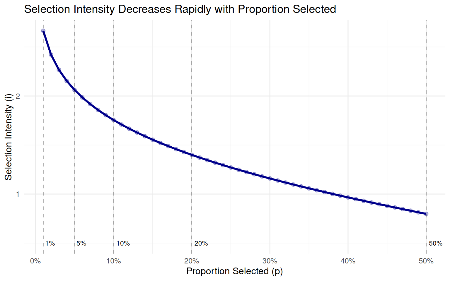
Notice the nonlinear relationship: intensity increases very rapidly as we become more selective. Going from 10% to 5% selected increases intensity by only 0.30 units, but going from 5% to 1% increases it by 0.61 units.
6.3.4 Example 1: Dairy Bull Selection Intensity
A dairy breeding company evaluates 1,000 young bulls each year using genomic selection. They want to select sires for widespread AI distribution. Let’s compare different selection intensities:
Scenario A: Select top 50 bulls (5%)
- p = 50/1000 = 0.05
- i = 2.06
Scenario B: Select top 100 bulls (10%)
- p = 100/1000 = 0.10
- i = 1.76
Difference in response: Using the same accuracy (r) and genetic parameters, Scenario A will achieve (2.06/1.76) = 1.17 times the response of Scenario B. By being twice as selective (5% vs 10%), they gain 17% more genetic progress.
However, Scenario A means: - Lower genetic diversity (more related bulls being used) - Higher risk of inbreeding - May not meet demand for semen from customers
This illustrates a common trade-off: intensity vs. genetic diversity.
6.3.5 Example 2: Swine Selection Intensity—Males vs. Females
In a swine breeding program, reproductive biology creates different opportunities for selection intensity in males versus females.
Male (boar) selection: - Evaluate 500 young boars annually - Select 10 for breeding (via AI) - p = 10/500 = 0.02 - i = 2.42 (very high intensity)
Female (gilt) selection: - Evaluate 2,000 young gilts annually - Select 400 to maintain herd size - p = 400/2,000 = 0.20 - i = 1.40 (moderate intensity)
The boars can be selected much more intensely because of AI—one boar can sire thousands of offspring. Each gilt can only produce 2-3 litters per year, so we need many more females to maintain the population.
The average selection intensity across sexes is:
\[ \bar{i} = \frac{i_{males} + i_{females}}{2} = \frac{2.42 + 1.40}{2} = 1.91 \]
This averaged intensity is what we’d use in the breeder’s equation to predict overall response to selection.
6.3.6 Factors Limiting Selection Intensity
While high intensity is desirable for maximizing genetic gain, several practical constraints limit how intensely we can select:
Reproductive capacity: We need enough parents to produce the next generation. Females have lower reproductive capacity than males (especially with AI), limiting female selection intensity.
Genetic diversity and inbreeding: Selecting very few parents reduces effective population size (Ne) and increases inbreeding. Most breeding programs aim to keep Ne ≥ 100 to maintain genetic diversity.
Economic constraints: Maintaining a breeding population costs money. Smaller populations (higher intensity) may have lower costs but higher genetic risks.
Market demand: For seedstock producers, customers want access to multiple elite sires. Selecting only 1-2 bulls might maximize intensity but won’t meet market needs.
Catastrophic risk: If all offspring come from a few parents and those parents carry an undetected lethal recessive, the consequences could be disastrous.
6.3.7 Species Differences in Selection Intensity
Different livestock species have different capacities for selection intensity:
| Species | Males (i) | Females (i) | Reason for Differences |
|---|---|---|---|
| Poultry (broilers/layers) | 2.5-2.7 | 2.0-2.2 | Very high reproductive rate, large populations |
| Swine | 2.2-2.5 | 1.3-1.5 | AI enables high male intensity; females moderate |
| Dairy cattle | 2.0-2.3 | 0.8-1.2 | AI enables high male intensity; all females needed |
| Beef cattle | 1.8-2.2 | 1.0-1.4 | Natural service limits male intensity; moderate female |
| Sheep | 1.8-2.2 | 1.2-1.6 | Moderate reproductive rate |
| Horses | 1.0-1.5 | 0.5-0.8 | Low reproductive rate, long generation interval |
Poultry can achieve the highest intensities due to: - Large population sizes (thousands of birds evaluated) - High reproductive rates (many eggs per hen) - Short generation intervals (rapid turnover)
Dairy cattle have asymmetric intensities: - High male intensity (AI from elite bulls) - Low female intensity (most/all cows retained for milk production)
Horses have the lowest intensities: - Low reproductive rates (one foal per mare per year) - Often breed for pedigree rather than performance - Natural mating is common (no AI in Thoroughbreds)
6.3.8 Calculating Selection Intensity in R
# Function to calculate selection intensity given proportion selected
# Based on truncation selection in a normal distribution
calculate_intensity <- function(p) {
  # Find the standardized threshold (z-score)
  threshold <- qnorm(1 - p)
  # Calculate intensity as mean of truncated normal
  intensity <- dnorm(threshold) / p
  return(intensity)
}

# Example: Calculate intensity for different proportions
proportions <- c(0.01, 0.05, 0.10, 0.20, 0.50)
intensities <- sapply(proportions, calculate_intensity)

intensity_results <- tibble(
  `Proportion Selected` = proportions,
  `Selection Intensity` = round(intensities, 2)
)

kable(intensity_results,
caption = "Calculated selection intensities")| Proportion Selected | Selection Intensity |
|---|---|
| 0.01 | 2.67 |
| 0.05 | 2.06 |
| 0.10 | 1.75 |
| 0.20 | 1.40 |
| 0.50 | 0.80 |
# Example: Swine breeding program
cat("\n--- Swine Breeding Program ---\n")
--- Swine Breeding Program ---cat("Male selection: 10 selected from 500 candidates\n")Male selection: 10 selected from 500 candidatesp_males <- 10/500
i_males <- calculate_intensity(p_males)
cat(" p =", p_males, " → i =", round(i_males, 2), "\n\n") p = 0.02 → i = 2.42 cat("Female selection: 400 selected from 2000 candidates\n")Female selection: 400 selected from 2000 candidatesp_females <- 400/2000
i_females <- calculate_intensity(p_females)
cat(" p =", p_females, " → i =", round(i_females, 2), "\n\n") p = 0.2 → i = 1.4 Average intensity: 1.91 6.4 Accuracy of Selection (r)
6.4.1 What Is Accuracy?
Accuracy of selection (r) measures how well we can predict true breeding values (TBV) from the information we have. It’s defined as the correlation between estimated breeding values (EBV) and true breeding values:
\[ r = \text{cor}(EBV, TBV) = \frac{\text{cov}(EBV, TBV)}{\sigma_{EBV} \times \sigma_{TBV}} \]
Accuracy ranges from 0 to 1: - r = 0: No information; EBVs are unrelated to TBVs (random selection) - r = 1: Perfect information; we know TBVs exactly (impossible in reality) - r = 0.50: Moderate information; EBVs explain 25% of variance in TBVs (r² = 0.25) - r = 0.90: High information; EBVs explain 81% of variance in TBVs (r² = 0.81)
Higher accuracy means we’re better at identifying the genetically superior animals, leading to more response to selection for the same selection intensity.
6.4.2 Why Accuracy Matters
Imagine you’re selecting bulls for dairy cattle breeding. You have 100 bulls to choose from, and you want to select the top 5 (i = 2.06). If your accuracy is low (r = 0.30), you’ll make many mistakes—animals you think are in the top 5 might actually be mediocre, and truly superior animals might be culled. If your accuracy is high (r = 0.85), you’ll correctly identify most of the truly elite bulls.
The impact of accuracy is multiplicative: doubling accuracy from r = 0.35 to r = 0.70 doubles the response to selection (assuming other factors remain constant).
6.4.3 Factors Affecting Accuracy
Four main factors determine accuracy:
- Heritability of the trait: Higher h² means individual records are more informative
- Amount of information: More records (own, progeny, relatives, genomic) increase accuracy
- Quality of information: Accurate measurements and proper contemporary grouping matter
- Relationship to animals with records: Closer relatives provide more information
1. Heritability and Accuracy
For selection based on an animal’s own phenotype, accuracy is related to heritability:
\[ r = \sqrt{h^2} \]
This means: - If h² = 0.36, then r = √0.36 = 0.60 - If h² = 0.81, then r = √0.81 = 0.90 - If h² = 0.09, then r = √0.09 = 0.30
Higher heritability traits allow higher accuracy from own performance.
# Create sequence of heritabilities
h2_values <- seq(0, 1, by = 0.01)
accuracy_values <- sqrt(h2_values)

ggplot(tibble(h2 = h2_values, accuracy = accuracy_values),
       aes(x = h2, y = accuracy)) +
  geom_line(color = "darkgreen", size = 1.2) +
  geom_hline(yintercept = c(0.3, 0.5, 0.7, 0.9),
             linetype = "dashed", alpha = 0.3) +
  annotate("text", x = 0.95, y = 0.3, label = "r = 0.30", hjust = 1) +
  annotate("text", x = 0.95, y = 0.5, label = "r = 0.50", hjust = 1) +
  annotate("text", x = 0.95, y = 0.7, label = "r = 0.70", hjust = 1) +
  annotate("text", x = 0.95, y = 0.9, label = "r = 0.90", hjust = 1) +
  scale_x_continuous(breaks = seq(0, 1, 0.1)) +
  scale_y_continuous(breaks = seq(0, 1, 0.1)) +
  labs(x = "Heritability (h²)",
       y = "Accuracy (r)",
       title = "Accuracy from Own Performance: r = √h²") +
  theme_minimal(base_size = 12)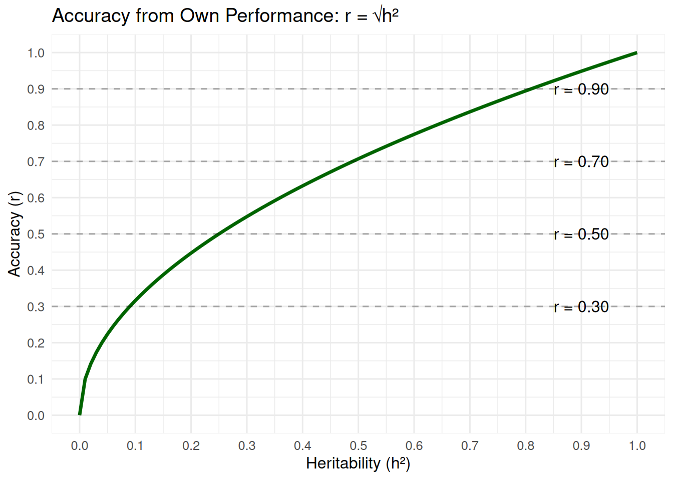
2. Amount of Information
As we gain more information about an animal or its relatives, accuracy increases. However, the relationship is not linear—each additional record adds less to accuracy than the previous one.
Information Sources for Accuracy
Own records: - Own phenotype (most basic) - Multiple repeated records (for repeatable traits like milk yield)
Pedigree information: - Parents’ EBVs (midparent breeding value) - Grandparents and more distant ancestors
Relatives’ records: - Full siblings (share 50% of genes) - Half siblings (share 25% of genes) - Progeny (each shares 50% of genes) - More progeny → higher accuracy
Genomic information: - 50,000+ SNP markers across the genome - Captures Mendelian sampling variation - Enables high accuracy at birth
6.4.4 Accuracy by Information Source
The table below shows typical accuracy values depending on the information available:
| Information Source | Typical Accuracy (r) | Notes |
|---|---|---|
| No information (population mean only) | 0.00 | Random selection |
| Pedigree only (midparent EBV) | 0.35-0.45 | Based on parents’ breeding values |
| Own performance (1 record, h² = 0.30) | 0.55 | Accuracy = √h² = √0.30 ≈ 0.55 |
| Own performance (3 repeated records) | 0.65-0.70 | Multiple records increase accuracy |
| Own + 10 progeny records | 0.75 | Progeny are highly informative |
| Own + 50 progeny records | 0.85 | Diminishing returns per progeny |
| Own + 100 progeny records | 0.88-0.90 | Approaching maximum |
| Genomic EBV (young animal, reference n=5,000) | 0.50-0.60 | Moderate accuracy without waiting |
| Genomic EBV (young animal, reference n=50,000) | 0.65-0.70 | Larger reference = higher accuracy |
| Genomic + progeny (ssGBLUP, 50 progeny) | 0.90-0.93 | Best of genomic and progeny info |
6.4.5 Example 3: Genomic vs. Progeny-Tested Bulls
A dairy breeding company must decide between two selection strategies for young bulls:
Strategy A: Progeny testing - Wait for each bull to produce ~50 daughters - Measure daughters’ milk yield over first lactation - Accuracy of EBV: r = 0.85 - Time required: 6 years (bulls at 2 years + daughters at 2 years + 2 years lactation)
Strategy B: Genomic selection - Genotype bulls at birth with 50K SNP chip - Calculate genomic EBV (GEBV) using reference population - Accuracy of GEBV: r = 0.65 - Time required: 0 years (selection at birth)
Which strategy gives more annual genetic gain? We’ll calculate this fully in Section 6.7, but notice that Strategy B has much lower generation interval (2.5 vs 6 years) even though accuracy is lower. The net effect is that genomic selection often wins despite lower accuracy.
6.4.6 Example 4: Broiler Trait Accuracy Comparison
Consider two traits in broiler chickens with different heritabilities:
Trait 1: Body weight at 42 days (high heritability) - h² = 0.40 - Accuracy from own performance: r = √0.40 = 0.63
Trait 2: Leg soundness score (moderate heritability) - h² = 0.22 - Accuracy from own performance: r = √0.22 = 0.47
For body weight, own performance gives good accuracy (0.63). For leg soundness, own performance gives lower accuracy (0.47), so progeny testing or genomic selection might be more valuable for this trait.
With genomic selection (assuming well-powered reference population): - Body weight GEBV accuracy: r ≈ 0.70 (marginal improvement over phenotype) - Leg soundness GEBV accuracy: r ≈ 0.55 (substantial improvement over phenotype)
This shows that genomic selection is most valuable for low heritability traits where phenotypic selection is least accurate.
6.4.7 Diminishing Returns from Additional Information
Let’s simulate how accuracy increases with the number of progeny records:
# Function to approximate accuracy with n progeny records
# Simplified formula: r = sqrt(n*h^2 / (4 + n*h^2))
# This is approximate for demonstration
accuracy_with_progeny <- function(n_progeny, h2) {
  # Approximate accuracy from n progeny
  # Based on half-sib family information
  r <- sqrt((n_progeny * h2/4) / (1 + (n_progeny - 1) * h2/4))
  return(r)
}

# Create data for different heritabilities
n_progeny_range <- 0:200
h2_levels <- c(0.10, 0.30, 0.50)

accuracy_data <- expand_grid(
  n_progeny = n_progeny_range,
  h2 = h2_levels
) %>%
  mutate(
    accuracy = map2_dbl(n_progeny, h2, accuracy_with_progeny),
    h2_label = paste0("h² = ", h2)
  )

ggplot(accuracy_data, aes(x = n_progeny, y = accuracy, color = h2_label)) +
  geom_line(size = 1.2) +
  geom_hline(yintercept = c(0.5, 0.7, 0.9),
             linetype = "dashed", alpha = 0.3) +
  scale_color_manual(values = c("darkred", "darkblue", "darkgreen")) +
  labs(x = "Number of Progeny Records",
       y = "Accuracy (r)",
       color = "Heritability",
       title = "Accuracy Increases with Progeny, But Diminishing Returns",
       subtitle = "Higher heritability traits reach high accuracy with fewer progeny") +
  theme_minimal(base_size = 12) +
  theme(legend.position = c(0.85, 0.25))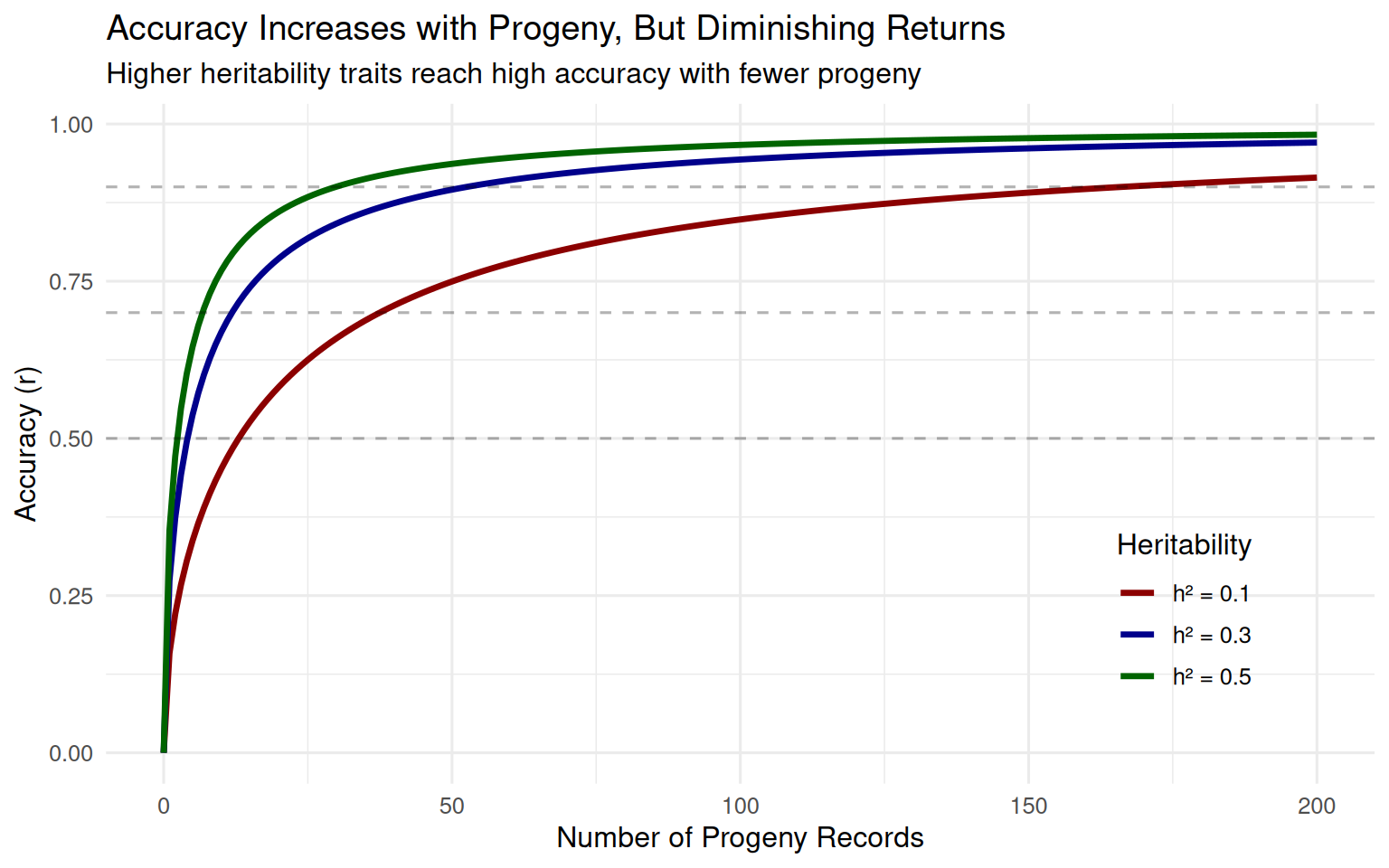
Key insights from this figure:
- Diminishing returns: The first 20 progeny add much more accuracy than progeny 100-120
- Higher h² helps: Traits with higher heritability reach high accuracy with fewer progeny
- Low h² traits are challenging: For h² = 0.10, even 200 progeny only gives r ≈ 0.70
This is why progeny testing is expensive and time-consuming for low heritability traits. Genomic selection provides an attractive alternative by achieving moderate accuracy without waiting for progeny.
6.4.8 Calculating Accuracy in R
# Accuracy from own performance
calculate_accuracy_own <- function(h2) {
  return(sqrt(h2))
}

# Example: Different heritabilities
h2_values <- c(0.10, 0.30, 0.50, 0.80)
accuracies <- calculate_accuracy_own(h2_values)

tibble(
  `Heritability (h²)` = h2_values,
  `Accuracy (r)` = round(accuracies, 3)
) %>%
kable(caption = "Accuracy from own performance for different heritabilities")| Heritability (h²) | Accuracy (r) |
|---|---|
| 0.1 | 0.316 |
| 0.3 | 0.548 |
| 0.5 | 0.707 |
| 0.8 | 0.894 |
6.5 Genetic Standard Deviation (σA)
6.5.1 What Is Genetic Standard Deviation?
The genetic standard deviation (σA) quantifies how much additive genetic variation exists in a population for a trait. It’s the standard deviation of true breeding values (TBVs) across all animals in the population.
Mathematically:
\[ \sigma_A = \sqrt{\sigma^2_A} = \sqrt{h^2 \times \sigma^2_P} \]
Where: - σ²A = additive genetic variance - σ²P = phenotypic variance - h² = heritability (narrow-sense)
6.5.2 Why σA Matters
Genetic standard deviation determines the ceiling for genetic improvement. If there’s no genetic variation (σA = 0), there’s no potential for selection to change the population mean, regardless of how intense or accurate our selection is.
Consider two populations:
Population A: Wide genetic variation (large σA) - Animals range from poor to excellent - Selection can choose truly superior animals - Large potential for genetic gain
Population B: Narrow genetic variation (small σA) - All animals are similar genetically - Selection has little to work with - Limited potential for genetic gain
6.5.3 Calculating σA from Variance Components
If we know the heritability and phenotypic variance for a trait, we can calculate σA:
\[ \sigma_A = \sqrt{h^2 \times \sigma^2_P} \]
Let’s use our variance components dataset to calculate σA for multiple traits across species.
6.5.4 Example 5: Calculating σA for Multiple Species and Traits
# Load variance components data (already loaded at top of chapter)
# Calculate sigma_A for each trait
variance_results <- variance_data %>%
  mutate(
    sigma_A = sqrt(sigma2_A),
    sigma_P = sqrt(sigma2_P)
  ) %>%
  select(species, trait, h2, sigma2_A, sigma_A, sigma_P)

# Display a subset of interesting comparisons
selected_traits <- variance_results %>%
  filter(
    trait %in% c("Milk_yield_kg", "Litter_size_total_born",
                 "Average_daily_gain_g", "Backfat_mm",
                 "Body_weight_42d_g", "Weaning_weight_kg",
                 "Fleece_weight_kg", "Body_weight_harvest_kg")
  ) %>%
  mutate(
    trait_clean = case_when(
      trait == "Milk_yield_kg" ~ "Milk yield (kg)",
      trait == "Litter_size_total_born" ~ "Litter size (pigs)",
      trait == "Average_daily_gain_g" ~ "Avg daily gain (g)",
      trait == "Backfat_mm" ~ "Backfat (mm)",
      trait == "Body_weight_42d_g" ~ "Body weight 42d (g)",
      trait == "Weaning_weight_kg" ~ "Weaning weight (kg)",
      trait == "Fleece_weight_kg" ~ "Fleece weight (kg)",
      trait == "Body_weight_harvest_kg" ~ "Harvest weight (kg)"
    )
  ) %>%
  select(Species = species,
         Trait = trait_clean,
         `h²` = h2,
         `σ²_A` = sigma2_A,
         `σ_A` = sigma_A,
         `σ_P` = sigma_P)

kable(selected_traits,
      digits = c(0, 0, 2, 1, 1, 1),
caption = "Genetic standard deviations for selected traits across species")| Species | Trait | h² | σ²_A | σ_A | σ_P |
|---|---|---|---|---|---|
| Dairy | Milk yield (kg) | 0.31 | 2.5e+05 | 500.0 | 894.4 |
| Swine | Litter size (pigs) | 0.11 | 8.0e-01 | 0.9 | 2.6 |
| Swine | Avg daily gain (g) | 0.40 | 1.2e+03 | 34.6 | 54.8 |
| Swine | Backfat (mm) | 0.42 | 2.5e+00 | 1.6 | 2.4 |
| Beef | Weaning weight (kg) | 0.38 | 1.8e+02 | 13.4 | 21.9 |
| Poultry_Broiler | Body weight 42d (g) | 0.40 | 1.8e+04 | 134.2 | 212.1 |
| Sheep | Weaning weight (kg) | 0.36 | 2.0e+00 | 1.4 | 2.3 |
| Sheep | Fleece weight (kg) | 0.44 | 3.0e-01 | 0.6 | 0.9 |
| Aquaculture_Salmon | Harvest weight (kg) | 0.33 | 1.0e-01 | 0.4 | 0.7 |
Interpretation of results:
-
Dairy milk yield: σA = 500 kg
- Large genetic variation in milk production
- Selection can make substantial gains in kg milk per lactation
-
Swine litter size: σA = 0.89 pigs
- Limited genetic variation
- Even with perfect selection, gains are small per generation
- This is why litter size improves slowly
-
Broiler body weight: σA = 134 g
- Moderate to high genetic variation
- Combined with high h², short L, and high i, leads to rapid progress
-
Swine backfat: σA = 1.58 mm
- Moderate genetic variation
- High h² makes this trait respond well to selection
6.5.5 Why We Can’t Easily Change σA
Unlike selection intensity, accuracy, and generation interval—all of which breeders can manipulate—σA is largely beyond our control. It’s determined by the population’s evolutionary history and current genetic diversity.
Factors that influence σA:
- Historical effective population size: Smaller populations have less genetic variation
- Past selection: Intense selection gradually reduces σA by fixing favorable alleles
- Mutation: Adds new variation, but very slowly (negligible over breeding program timescales)
- Migration/crossbreeding: Introducing new genetics can increase σA
- Number of loci affecting the trait: More loci generally means more sustained variation
In closed breeding populations (common in livestock), σA typically decreases slowly over time as selection fixes favorable alleles and inbreeding occurs. However, this decrease is usually small over 10-20 generations.
6.5.6 Response to Selection Depends Heavily on σA
Let’s compare expected response for two traits with very different genetic standard deviations, holding other factors constant:
Trait A: High genetic variation - i = 2.0 - r = 0.65 - σA = 150 kg - L = 2 years - R = (2.0 × 0.65 × 150) / 2 = 97.5 kg per year
Trait B: Low genetic variation - i = 2.0 - r = 0.65 - σA = 15 kg (10× smaller) - L = 2 years - R = (2.0 × 0.65 × 15) / 2 = 9.75 kg per year (10× smaller)
Even with identical breeding program parameters (i, r, L), Trait A improves 10 times faster simply because it has more genetic variation to work with.
6.5.7 Visualizing Genetic Variation
# Simulate two populations with different sigma_A
set.seed(123)
n <- 1000

# Population 1: High genetic variation
pop1_tbv <- rnorm(n, mean = 100, sd = 20)  # sigma_A = 20
pop1_data <- tibble(
  TBV = pop1_tbv,
  Population = "High σ_A = 20"
)

# Population 2: Low genetic variation
pop2_tbv <- rnorm(n, mean = 100, sd = 5)   # sigma_A = 5
pop2_data <- tibble(
  TBV = pop2_tbv,
  Population = "Low σ_A = 5"
)

# Combine
variation_data <- bind_rows(pop1_data, pop2_data)

# Plot distributions
ggplot(variation_data, aes(x = TBV, fill = Population)) +
  geom_density(alpha = 0.6) +
  geom_vline(xintercept = 100, linetype = "dashed") +
  scale_fill_manual(values = c("darkblue", "darkred")) +
  labs(x = "True Breeding Value (TBV)",
       y = "Density",
       title = "Effect of Genetic Standard Deviation on Population Variation",
       subtitle = "Higher σ_A means more spread in breeding values → more potential for selection",
       fill = "Population") +
  theme_minimal(base_size = 12) +
  theme(legend.position = c(0.85, 0.85))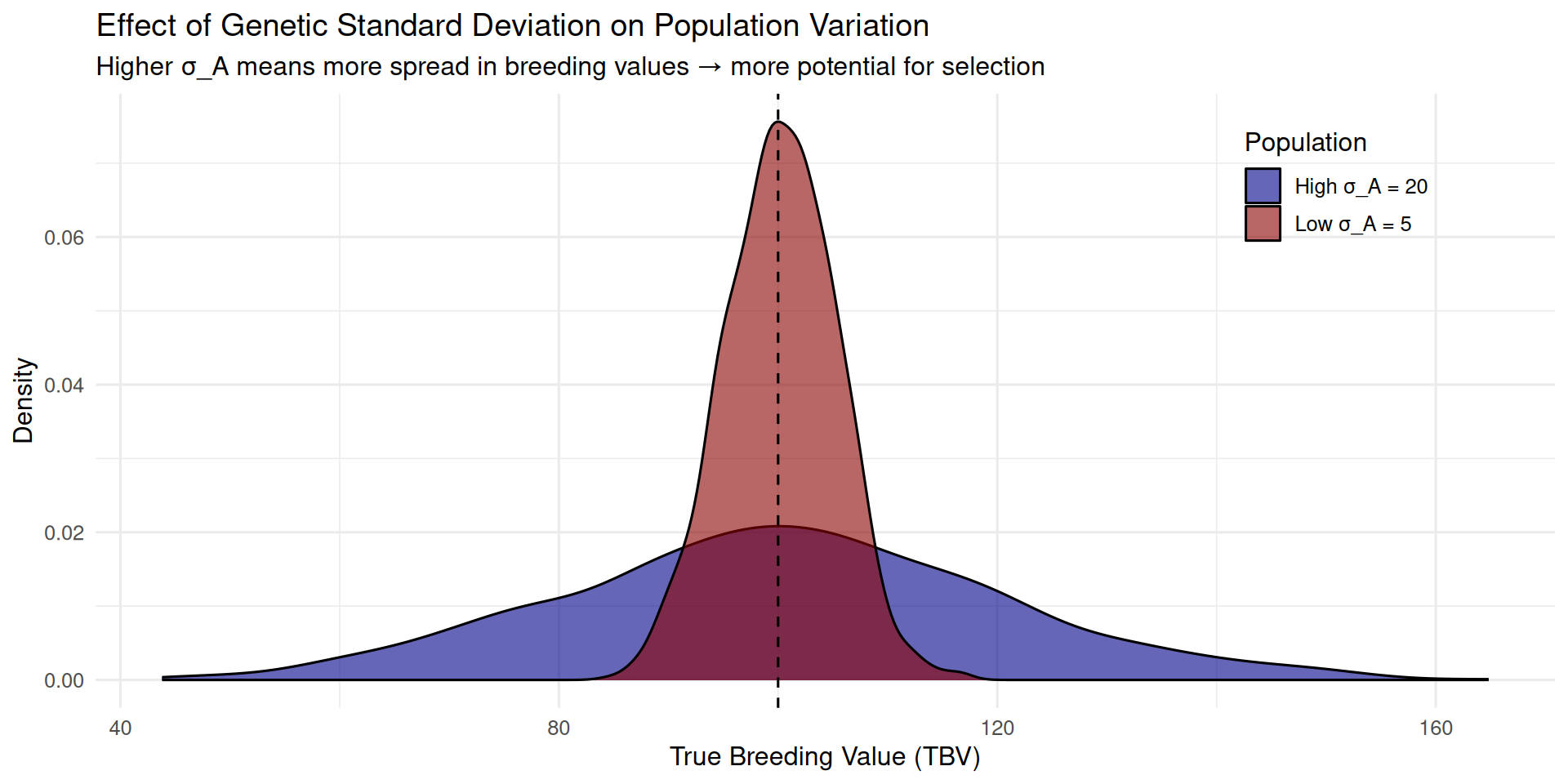
In the high σA population, there are many animals far above the mean—these are the genetic elite we want to select. In the low σA population, almost all animals cluster near the mean, so even intense selection yields modest gains.
6.5.8 Summary Table: Genetic Parameters Across Species
| Species | Traits Examined | Mean h² | Min σ_A | Max σ_A |
|---|---|---|---|---|
| Horse_Warmblood | 2 | 0.34 | 0.4 | 0.4 |
| Beef | 8 | 0.34 | 0.2 | 21.2 |
| Sheep | 5 | 0.34 | 0.3 | 1.7 |
| Poultry_Broiler | 5 | 0.32 | 0.1 | 134.2 |
| Aquaculture_Salmon | 3 | 0.30 | 0.2 | 0.5 |
| Poultry_Layer | 5 | 0.29 | 0.5 | 11.0 |
| Swine | 8 | 0.27 | 0.1 | 38.7 |
| Dairy | 6 | 0.23 | 0.3 | 500.0 |
| Horse_Thoroughbred | 2 | 0.20 | 0.3 | 109.5 |
6.6 Generation Interval (L)
6.6.1 What Is Generation Interval?
Generation interval (L) is the average age of parents when their offspring are born. It’s a critical factor because it determines how quickly we can accumulate genetic gains over time.
Formally:
\[ L = \frac{L_{\text{sires}} + L_{\text{dams}}}{2} \]
Where: - Lsires = average age of sires when offspring are born - Ldams = average age of dams when offspring are born
In some cases, these can differ substantially. For example, in dairy cattle, proven bulls might be used for 5-10 years (Lsires ≈ 7-8 years), while cows have their first calf at 2 years and may be in the herd for many lactations (Ldams ≈ 4-5 years).
6.6.2 Why Generation Interval Matters
The breeder’s equation calculates response per generation. To get annual response, we divide by L:
\[ R_{\text{per year}} = \frac{i \times r \times \sigma_A}{L} \]
A breeding program with L = 2 years will accumulate genetic gains 4 times faster than a program with L = 8 years, assuming all else is equal.
Consider two identical breeding programs, differing only in generation interval:
Program A: L = 2 years - Response per generation = 100 kg - Response per year = 100 / 2 = 50 kg/year - Over 20 years: 20 × 50 = 1,000 kg total gain
Program B: L = 8 years - Response per generation = 100 kg - Response per year = 100 / 8 = 12.5 kg/year - Over 20 years: 20 × 12.5 = 250 kg total gain
Program A achieves 4 times more genetic improvement in the same time period, purely because of faster generation turnover.
6.6.3 Example 6: Generation Interval by Species
Different livestock species have vastly different generation intervals due to: - Age at sexual maturity - Gestation length - Time needed to collect information (progeny testing) - Economic factors (when animals are most profitable)
| Species | Breeding Scheme | L_sires (years) | L_dams (years) | Average L (years) | Notes |
|---|---|---|---|---|---|
| Poultry (broilers) | Genomic selection | 1.0 | 1.0 | 1.00 | Rapid turnover, high throughput |
| Poultry (layers) | Genomic selection | 1.0 | 1.0 | 1.00 | Select annually on genomic EBVs |
| Swine | Phenotypic selection | 1.5 | 2.0 | 1.75 | Select on own performance at 6mo |
| Swine | Genomic selection | 1.0 | 1.5 | 1.25 | Select at birth using GEBVs |
| Sheep | Mixed | 2.5 | 3.5 | 3.00 | Varies by system and trait |
| Dairy cattle (pre-genomic) | Progeny testing | 7.0 | 5.0 | 6.00 | Bulls used at 7+, cows at 5 |
| Dairy cattle (genomic) | Genomic selection | 2.5 | 4.0 | 3.25 | Bulls used at 2-3, cows at 4 |
| Beef cattle | Natural service | 4.0 | 5.0 | 4.50 | Bulls used young, cows longer |
| Horses | Traditional | 10.0 | 10.0 | 10.00 | Show/race results needed, low repro |
Key observations:
Poultry has the shortest L: Birds can reproduce at ~6 months, and with genomic selection, breeding decisions are made at hatch. This is a major reason why poultry breeding programs achieve the fastest genetic gains.
Dairy cattle (pre-genomic) had long L: Waiting for progeny test results meant bulls weren’t widely used until 7+ years old. Genomic selection cut this in half by enabling selection at birth.
Horses have very long L: Low reproductive rates, long generation times, and selection often based on performance records (racing, showing) accumulated over years.
Genomic selection reduces L: Across all species, genomic selection enables earlier selection decisions by providing moderate-to-high accuracy EBVs at birth.
6.6.4 Factors Affecting Generation Interval
Several biological and economic factors determine L:
Biological factors: 1. Age at sexual maturity: Species mature at different rates 2. Gestation length: Longer gestation delays first offspring 3. Reproductive rate: Species with lower rates may keep animals longer
Information factors: 4. Time to collect phenotypes: Traits expressed late in life (longevity, lifetime production) increase L 5. Progeny testing: Waiting for offspring performance adds 1+ generations to L 6. Genomic selection: Enables selection at birth, minimizing L
Economic factors: 7. Cost of maintaining candidates: Cheaper to maintain → can afford shorter L 8. Value of production: In dairy, cows produce milk while breeding, justifying longer L 9. Facility constraints: Limited space may force longer L
6.6.5 The Trade-off: Accuracy vs. Generation Interval
The most fundamental trade-off in animal breeding is between accuracy (r) and generation interval (L):
Progeny testing: - ✓ High accuracy (r = 0.80-0.95) - ✗ Long generation interval (L increases by 4-6 years)
Genomic selection: - ✓ Short generation interval (L minimized, selection at birth) - ✗ Moderate accuracy (r = 0.50-0.70)
The key question: Is the gain in accuracy worth the cost in generation interval?
Let’s calculate this for a dairy cattle example:
Progeny testing: - i = 2.0, r = 0.90, σA = 500 kg, L = 6 years - R = (2.0 × 0.90 × 500) / 6 = 150 kg/year
Genomic selection: - i = 2.0, r = 0.65, σA = 500 kg, L = 2.5 years - R = (2.0 × 0.65 × 500) / 2.5 = 260 kg/year
Despite having much lower accuracy (0.65 vs 0.90), genomic selection achieves 73% higher annual genetic gain because of the dramatically shorter generation interval.
This calculation revolutionized dairy cattle breeding. Since ~2009, genomic selection has largely replaced progeny testing for most traits, roughly doubling the rate of genetic improvement.
6.6.6 Visualizing the Impact of Generation Interval
# Simulate genetic gain over 30 years for different generation intervals
years <- 0:30

# Assume response per generation = 100 units (same for all)
R_per_gen <- 100

# Different generation intervals
L_values <- c(1, 2, 4, 6, 8)

# Calculate cumulative response for each L
gen_interval_data <- expand_grid(
  year = years,
  L = L_values
) %>%
  mutate(
    # Number of generations completed by this year
    n_generations = year / L,
    # Cumulative genetic gain
    cumulative_gain = n_generations * R_per_gen,
    L_label = paste0("L = ", L, " years")
  )

# Plot
ggplot(gen_interval_data, aes(x = year, y = cumulative_gain,
                               color = L_label, group = L_label)) +
  geom_line(size = 1.2) +
  geom_point(size = 2, alpha = 0.5) +
  scale_color_viridis_d(option = "plasma", direction = -1) +
  labs(x = "Years",
       y = "Cumulative Genetic Gain (units)",
       color = "Generation\nInterval",
       title = "Shorter Generation Intervals Accumulate Gains Much Faster",
       subtitle = "Assuming equal response per generation (R = 100 units)") +
  theme_minimal(base_size = 12) +
  theme(legend.position = c(0.15, 0.75))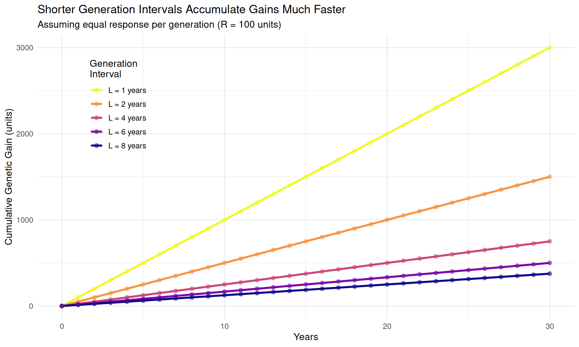
Interpretation: After 30 years: - L = 1 year: 3,000 units of gain (30 generations) - L = 2 years: 1,500 units of gain (15 generations) - L = 4 years: 750 units of gain (7.5 generations) - L = 8 years: 375 units of gain (3.75 generations)
The L = 1 year program achieves 8 times more improvement than the L = 8 year program, despite identical response per generation.
6.6.7 Calculating Generation Interval in R
# Function to calculate average generation interval
calculate_L <- function(L_sires, L_dams) {
  L <- (L_sires + L_dams) / 2
  return(L)
}

# Example: Dairy cattle breeding programs
cat("--- Dairy Cattle Generation Intervals ---\n\n")
--- Dairy Cattle Generation Intervals ---cat("Pre-genomic era (progeny testing):\n")Pre-genomic era (progeny testing):L_pre_genomic <- calculate_L(L_sires = 7, L_dams = 5)
cat(" L_sires = 7 years, L_dams = 5 years\n") L_sires = 7 years, L_dams = 5 yearscat(" Average L =", L_pre_genomic, "years\n\n") Average L = 6 yearscat("Genomic era:\n")Genomic era:L_genomic <- calculate_L(L_sires = 2.5, L_dams = 4)
cat(" L_sires = 2.5 years, L_dams = 4 years\n") L_sires = 2.5 years, L_dams = 4 yearscat(" Average L =", L_genomic, "years\n\n") Average L = 3.25 yearscat("Reduction in L:", L_pre_genomic - L_genomic, "years\n")Reduction in L: 2.75 yearsSpeed-up factor: 1.85 x6.7 Putting It All Together: Complete Examples
Now that we understand each component of the breeder’s equation, let’s work through complete examples for different species, calculating expected response to selection from start to finish.
6.7.1 Example 7: Dairy Cattle Milk Yield
Situation: A dairy breeding company wants to predict genetic gain for milk yield using genomic selection.
Step 1: Gather genetic parameters
From our variance components dataset:
# Extract dairy milk yield parameters
dairy_milk <- variance_data %>%
  filter(species == "Dairy", trait == "Milk_yield_kg")

h2_milk <- dairy_milk$h2
sigma2_A_milk <- dairy_milk$sigma2_A
sigma_A_milk <- sqrt(sigma2_A_milk)

cat("Milk yield genetic parameters:\n")
Milk yield genetic parameters:cat(" h² =", h2_milk, "\n") h² = 0.31 cat(" σ²_A =", sigma2_A_milk, "kg²\n") σ²_A = 250000 kg² σ_A = 500 kgStep 2: Determine breeding program parameters
Genomic selection program: - Select top 5% of bulls based on genomic EBVs: i = 2.06 - Genomic EBV accuracy (well-powered reference): r = 0.70 - Bulls used at 2.5 years, cows first calve at 2 years: L = (2.5 + 4)/2 = 3.25 years
Step 3: Calculate response to selection
# Breeding program parameters
i_bulls <- 2.06
r_genomic <- 0.70
L_genomic <- 3.25

# Calculate annual response
R_annual <- (i_bulls * r_genomic * sigma_A_milk) / L_genomic

cat("Expected response to selection:\n")
Expected response to selection:cat(" R = (i × r × σ_A) / L\n") R = (i × r × σ_A) / L R = ( 2.06 × 0.7 × 500 ) / 3.25 R = 221.8 kg per year# Calculate cumulative gain over 10 years
gain_10yr <- R_annual * 10
cat("Cumulative gain over 10 years:", round(gain_10yr, 0), "kg\n")Cumulative gain over 10 years: 2218 kg (That's about 0.2 kg per day!)Interpretation: This dairy breeding program expects to improve milk yield by approximately 222 kg per cow per lactation each year. Over a decade, this compounds to 2218 kg of genetic improvement—a substantial increase in production!
6.7.2 Example 8: Swine Litter Size
Situation: A swine breeding company wants to improve litter size (total pigs born). This is a challenging trait due to low heritability.
Step 1: Genetic parameters
# Extract swine litter size parameters
swine_litter <- variance_data %>%
  filter(species == "Swine", trait == "Litter_size_total_born")

h2_litter <- swine_litter$h2
sigma2_A_litter <- swine_litter$sigma2_A
sigma_A_litter <- sqrt(sigma2_A_litter)

cat("Litter size genetic parameters:\n")
Litter size genetic parameters:cat(" h² =", h2_litter, "(low heritability)\n") h² = 0.11 (low heritability)cat(" σ²_A =", sigma2_A_litter, "pigs²\n") σ²_A = 0.8 pigs² σ_A = 0.89 pigsStep 2: Breeding program parameters
- Select top 10% of boars: imales = 1.76
- Select top 20% of gilts: ifemales = 1.40
- Average intensity: iavg = (1.76 + 1.40)/2 = 1.58
- Accuracy with genomic selection: r = 0.45 (lower than high-h² traits)
- Generation interval: L = 1.75 years
Step 3: Calculate response
# Breeding program parameters
i_avg_swine <- 1.58
r_litter <- 0.45
L_swine <- 1.75

# Calculate annual response
R_litter <- (i_avg_swine * r_litter * sigma_A_litter) / L_swine

cat("Expected response to selection for litter size:\n")
Expected response to selection for litter size: R = ( 1.58 × 0.45 × 0.89 ) / 1.75 R = 0.363 pigs per year# Calculate cumulative gain over 10 years
gain_10yr_litter <- R_litter * 10
cat("Cumulative gain over 10 years:", round(gain_10yr_litter, 2), "pigs per litter\n")Cumulative gain over 10 years: 3.63 pigs per litterInterpretation: Litter size improves by only 0.363 pigs per year—much slower than high-heritability traits. This is due to: 1. Low heritability (h² = 0.11) → low σA 2. Low accuracy (r = 0.45) even with genomic selection 3. Low σA × moderate accuracy = small response
Even over 10 years, we only gain about 3.6 pig per litter. This illustrates why reproductive traits are slow to improve despite intensive selection.
6.7.3 Example 9: Broiler Body Weight
Situation: A poultry breeding company selecting for increased body weight at 42 days.
Step 1: Genetic parameters
# Extract broiler body weight parameters
broiler_bw <- variance_data %>%
  filter(species == "Poultry_Broiler", trait == "Body_weight_42d_g")

h2_broiler <- broiler_bw$h2
sigma2_A_broiler <- broiler_bw$sigma2_A
sigma_A_broiler <- sqrt(sigma2_A_broiler)

cat("Broiler body weight genetic parameters:\n")
Broiler body weight genetic parameters:cat(" h² =", h2_broiler, "\n") h² = 0.4 cat(" σ²_A =", sigma2_A_broiler, "g²\n") σ²_A = 18000 g² σ_A = 134.2 gStep 2: Breeding program parameters
Poultry breeding has unique advantages: - Very high selection intensity: i = 2.60 (top 1% selected, large populations) - Good accuracy with genomics: r = 0.70 - Very short generation interval: L = 1.0 year
Step 3: Calculate response
# Breeding program parameters
i_broiler <- 2.60
r_broiler <- 0.70
L_broiler <- 1.0

# Calculate annual response
R_broiler <- (i_broiler * r_broiler * sigma_A_broiler) / L_broiler

cat("Expected response to selection for broiler body weight:\n")
Expected response to selection for broiler body weight: R = ( 2.6 × 0.7 × 134.2 ) / 1 R = 244.2 grams per year# Calculate cumulative gain over 10 years
gain_10yr_broiler <- R_broiler * 10
cat("Cumulative gain over 10 years:", round(gain_10yr_broiler, 0), "grams (=",
round(gain_10yr_broiler/1000, 2), "kg)\n")Cumulative gain over 10 years: 2442 grams (= 2.44 kg)Interpretation: Broiler body weight improves by 244 grams per year—very rapid progress! This is due to the combination of all four favorable factors: 1. High selection intensity (i = 2.60) 2. Good accuracy (r = 0.70) 3. Substantial genetic variation (σA = 134 g) 4. Very short generation interval (L = 1 year)
Over 10 years, broilers gain nearly 2 kg of body weight from genetic improvement alone. This is why modern broilers grow so much faster than broilers from 30-40 years ago.
6.7.4 Example 10: Beef Cattle Weaning Weight
Situation: A beef cattle seedstock producer selecting for increased weaning weight.
Step 1: Genetic parameters
# Extract beef weaning weight parameters
beef_ww <- variance_data %>%
  filter(species == "Beef", trait == "Weaning_weight_kg")

h2_beef <- beef_ww$h2
sigma2_A_beef <- beef_ww$sigma2_A
sigma_A_beef <- sqrt(sigma2_A_beef)

cat("Beef weaning weight genetic parameters:\n")
Beef weaning weight genetic parameters:cat(" h² =", h2_beef, "\n") h² = 0.38 cat(" σ²_A =", sigma2_A_beef, "kg²\n") σ²_A = 180 kg² σ_A = 13.4 kgStep 2: Breeding program parameters
- Moderate selection intensity: i = 1.80 (top 8% of bulls, top 15% of cows, average ≈ 1.80)
- Good accuracy with genomic EPDs: r = 0.65
- Longer generation interval: L = 5.0 years (bulls at 3-4 years, cows at 6+ years average)
Step 3: Calculate response
# Breeding program parameters
i_beef <- 1.80
r_beef <- 0.65
L_beef <- 5.0

# Calculate annual response
R_beef <- (i_beef * r_beef * sigma_A_beef) / L_beef

cat("Expected response to selection for beef weaning weight:\n")
Expected response to selection for beef weaning weight: R = ( 1.8 × 0.65 × 13.4 ) / 5 R = 3.14 kg per year# Calculate cumulative gain over 20 years
gain_20yr_beef <- R_beef * 20
cat("Cumulative gain over 20 years:", round(gain_20yr_beef, 1), "kg\n")Cumulative gain over 20 years: 62.8 kgInterpretation: Beef weaning weight improves by about 3.1 kg per year—much slower than broilers or swine, primarily due to the long generation interval (L = 5 years). Even with favorable genetics (high h², good accuracy), the slow generational turnover limits annual progress.
6.7.5 Comparing the Four Species Examples
Let’s summarize and compare our four examples:
| Species | Trait | i | r | σ_A | L | R (per year) | Key Limiting Factor |
|---|---|---|---|---|---|---|---|
| Dairy cattle | Milk yield | 2.06 | 0.70 | 500 kg | 3.25 | 221.800 | Moderate L |
| Swine | Litter size | 1.58 | 0.45 | 0.89 pigs | 1.75 | 0.362 | Low h² → low σ_A and r |
| Broilers | Body weight 42d | 2.60 | 0.70 | 134 g | 1.00 | 244.200 | None (all factors favorable) |
| Beef cattle | Weaning weight | 1.80 | 0.65 | 13.4 kg | 5.00 | 3.140 | Long L |
Key insights:
- Broilers achieve fastest progress: All four factors work in their favor
- Swine litter size improves slowly: Low heritability is the limiting factor
- Beef cattle held back by L: Good genetics, but generational turnover is slow
- Dairy cattle moderate progress: Genomic selection helped, but L still substantial
6.8 Comparing Selection Strategies
The breeder’s equation is most powerful when used to compare alternative breeding strategies. Should we progeny test or use genomic selection? Should we measure a difficult trait or rely on correlated traits? These decisions can be informed by calculating expected response under each scenario.
6.8.1 Three Common Selection Strategies
Let’s define three selection strategies that differ in how they achieve accuracy:
Strategy 1: Mass Selection (Own Performance) - Select animals based on their own phenotype - Accuracy: r = √h² - Generation interval: Minimal (select as soon as trait is measured) - No progeny information needed
Strategy 2: Progeny Testing - Wait for offspring to be born and measured - Accuracy: r = 0.80-0.95 (depending on number of progeny) - Generation interval: Long (adds 1-2 generations to L) - Expensive and time-consuming
Strategy 3: Genomic Selection - Genotype at birth, predict breeding value from DNA - Accuracy: r = 0.50-0.75 (depending on trait and reference population) - Generation interval: Minimal (select at birth) - Requires genomic infrastructure and reference population
6.8.2 Example 11: Dairy Bull Selection—Comparing All Three Strategies
Let’s compare these three strategies for selecting dairy bulls for milk yield:
Common parameters: - Selection intensity: i = 2.06 (top 5% selected) - Genetic standard deviation: σA = 500 kg - Trait heritability: h² = 0.31
Strategy 1: Mass selection (own performance)
Wait, bulls don’t produce milk! For dairy bulls, we can’t use mass selection for milk yield. We’d need to use dam’s milk yield or midparent breeding value, which gives r ≈ 0.40.
- r = 0.40 (based on parents’ EBVs)
- L = 2.5 years (select bulls based on parents when bulls reach breeding age)
# Strategy 1: Selection on parental information
i <- 2.06
r_parent <- 0.40
sigma_A <- 500
L_parent <- 2.5

R_parent <- (i * r_parent * sigma_A) / L_parent
cat("Strategy 1 - Parent-based selection:\n")
Strategy 1 - Parent-based selection: R = 164.8 kg/yearStrategy 2: Progeny testing
Wait for 50-100 daughters to complete first lactation: - r = 0.90 (high accuracy from many progeny) - L = 7.0 years (bulls at 2 + daughters at 2 + 1 year lactation + time to evaluate = 7 years to first widespread use)
# Strategy 2: Progeny testing
r_progeny <- 0.90
L_progeny <- 7.0

R_progeny <- (i * r_progeny * sigma_A) / L_progeny
cat("Strategy 2 - Progeny testing:\n")
Strategy 2 - Progeny testing: R = 132.4 kg/yearStrategy 3: Genomic selection
Genotype at birth, calculate GEBV: - r = 0.70 (good accuracy with large reference population) - L = 2.5 years (select based on GEBV, use bulls at maturity)
# Strategy 3: Genomic selection
r_genomic <- 0.70
L_genomic <- 2.5

R_genomic <- (i * r_genomic * sigma_A) / L_genomic
cat("Strategy 3 - Genomic selection:\n")
Strategy 3 - Genomic selection: R = 288.4 kg/yearSummary and comparison:
# Create comparison table
strategy_comparison <- tibble(
  Strategy = c("Parent-based", "Progeny testing", "Genomic selection"),
  Accuracy_r = c(r_parent, r_progeny, r_genomic),
  Gen_interval_L = c(L_parent, L_progeny, L_genomic),
  Response_per_year = c(R_parent, R_progeny, R_genomic),
  Relative_to_progeny = c(R_parent/R_progeny, 1, R_genomic/R_progeny)
)

kable(strategy_comparison,
      digits = c(0, 2, 1, 1, 2),
      col.names = c("Strategy", "Accuracy (r)", "Gen. Interval (L)",
                    "Response (kg/yr)", "Relative to Progeny Test"),
caption = "Comparison of three selection strategies for dairy milk yield")| Strategy | Accuracy (r) | Gen. Interval (L) | Response (kg/yr) | Relative to Progeny Test |
|---|---|---|---|---|
| Parent-based | 0.4 | 2.5 | 164.8 | 1.24 |
| Progeny testing | 0.9 | 7.0 | 132.4 | 1.00 |
| Genomic selection | 0.7 | 2.5 | 288.4 | 2.18 |
Interpretation:
Progeny testing has the highest accuracy (0.90) but long generation interval (7 years) → R = 132 kg/year
-
Genomic selection has lower accuracy (0.70) but much shorter L (2.5 years) → R = 288 kg/year
- 2.18× faster than progeny testing!
-
Parent-based selection is fastest (L = 2.5) but lowest accuracy (0.40) → R = 165 kg/year
- Still better than progeny testing due to much shorter L
This analysis explains why genomic selection revolutionized dairy cattle breeding around 2009. By achieving good accuracy without the long generation interval required for progeny testing, genomic selection roughly doubled the annual rate of genetic gain.
6.8.3 Visualizing Strategy Comparison
Let’s plot the cumulative genetic progress over 20 years for each strategy:
# Simulate genetic trends for each strategy
years <- 0:20

strategy_trends <- tibble(
  Year = rep(years, 3),
  Strategy = rep(c("Parent-based", "Progeny Testing", "Genomic Selection"),
                 each = length(years)),
  Annual_Response = rep(c(R_parent, R_progeny, R_genomic), each = length(years))
) %>%
  mutate(
    Cumulative_Gain = Year * Annual_Response
  )

ggplot(strategy_trends, aes(x = Year, y = Cumulative_Gain,
                            color = Strategy, linetype = Strategy)) +
  geom_line(size = 1.3) +
  geom_point(size = 2.5, alpha = 0.6) +
  scale_color_manual(values = c("Parent-based" = "orange",
                                 "Progeny Testing" = "darkred",
                                 "Genomic Selection" = "darkblue")) +
  scale_linetype_manual(values = c("Parent-based" = "dotted",
                                    "Progeny Testing" = "dashed",
                                    "Genomic Selection" = "solid")) +
  labs(x = "Years Since Program Start",
       y = "Cumulative Genetic Gain (kg milk)",
       title = "Genomic Selection Achieves Much Faster Cumulative Progress",
       subtitle = "Despite lower accuracy, short generation interval dominates") +
  theme_minimal(base_size = 12) +
  theme(legend.position = c(0.2, 0.8))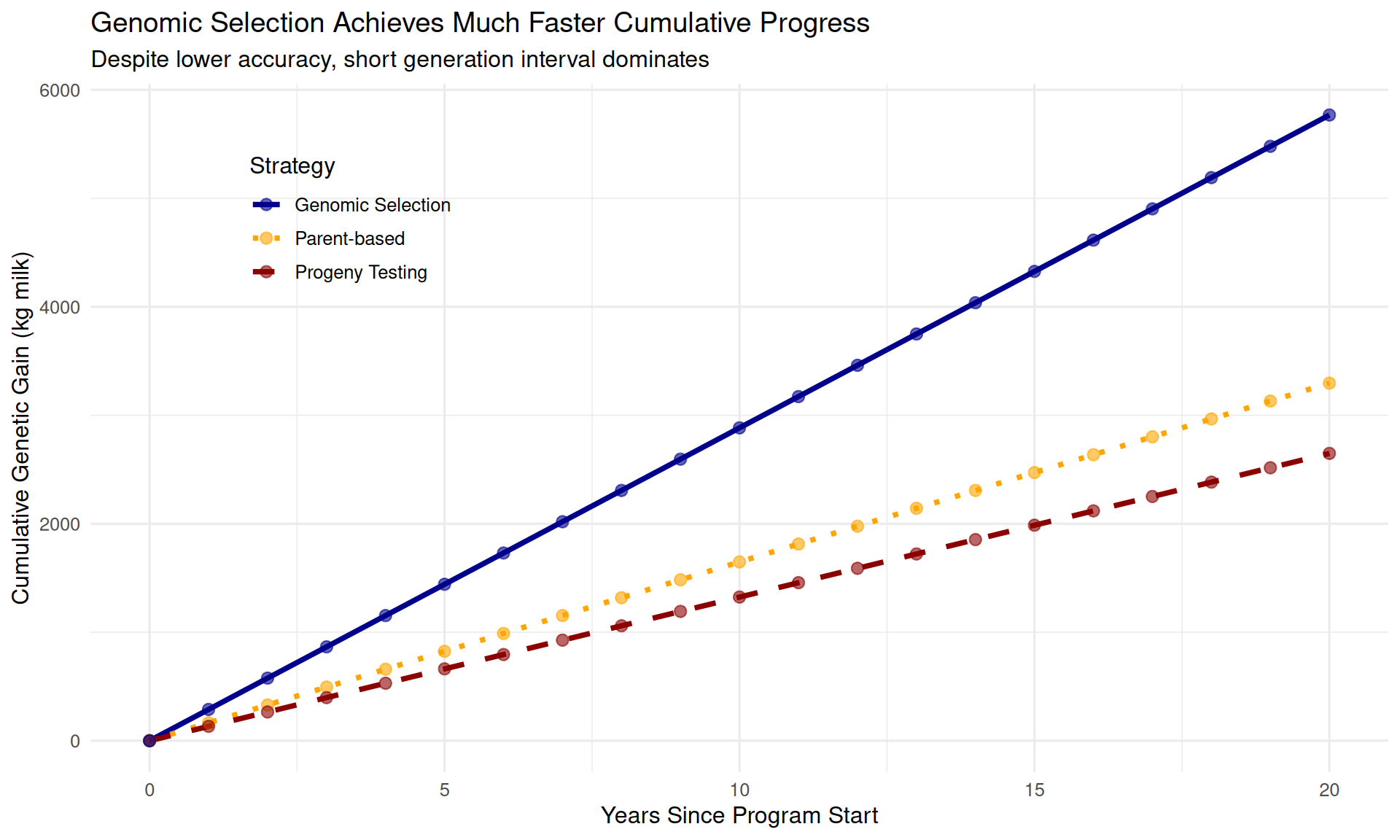
After 20 years: - Genomic selection: 5768 kg cumulative gain - Progeny testing: 2649 kg cumulative gain - Parent-based: 3296 kg cumulative gain
Genomic selection achieves 2.2× more progress than progeny testing over 20 years!
6.8.4 Economic Considerations
Annual genetic response isn’t the only factor—we must also consider costs:
Progeny testing costs: - Maintaining daughters in test herds - Recording and analyzing data - Storing semen while waiting for results - Opportunity cost of delayed selection
Genomic selection costs: - Initial: Building reference population (genotyping + phenotyping thousands of animals) - Ongoing: Genotyping all selection candidates ($30-150 per animal) - Updating reference population regularly - Bioinformatics infrastructure
For traits that are expensive or difficult to measure (e.g., feed efficiency, disease resistance, carcass traits), genomic selection has an even bigger advantage—it can achieve moderate accuracy at birth for traits that would be very costly to phenotype on all candidates.
6.9 Trade-offs Among the Four Factors
The four factors in the breeder’s equation are not independent. Optimizing one factor often requires compromises in others. Understanding these trade-offs is essential for designing effective breeding programs.
6.9.1 The Classic Trade-off: Accuracy vs. Generation Interval
This is the most important trade-off in animal breeding:
To increase accuracy: - Collect more phenotypic data (takes time) - Wait for progeny records (adds 1-2 generations) - Measure traits late in life (increases L)
To decrease generation interval: - Select animals young (less information, lower accuracy) - Make decisions quickly (less certainty)
The tension: Higher accuracy requires more time, increasing L. Lower L means making decisions with less information, reducing r.

Key insight: Before genomic selection, breeders faced a hard choice: accept lower accuracy (select young) or accept longer generation intervals (progeny test). Genomic selection breaks this trade-off by providing good accuracy at birth.
6.9.2 Intensity vs. Genetic Diversity
Higher selection intensity (lower p) increases i and thus response to selection. However:
Consequences of very high intensity: 1. Reduced effective population size (Ne): Fewer parents → more inbreeding 2. Increased inbreeding coefficient (F): Related animals are mated 3. Inbreeding depression: Reduced fitness, fertility, health in inbred offspring 4. Loss of genetic diversity: Some favorable alleles may be lost by chance
Most breeding programs aim to balance intensity with diversity management: - Target Ne ≥ 100 (minimum for maintaining diversity) - Use optimum contribution selection (OCS) to maximize genetic gain while constraining inbreeding - Monitor inbreeding coefficient over time
Example: A swine breeding company could select only 2 boars (p = 0.002, i = 2.90), but this would: - Create very high inbreeding in next generation - Risk losing genetic diversity - Potentially expose hidden lethal recessives
Instead, they select 10-15 boars (p = 0.01-0.015, i = 2.4-2.7), accepting slightly lower intensity to maintain diversity.
6.9.3 Intensity vs. Generation Interval (Reproduction Constraints)
High intensity requires selecting very few animals, which means each parent must produce many offspring. This can increase generation interval:
Example in beef cattle: - To select top 1% of bulls (i = 2.67), each bull must sire ~100 calves - Using natural service, one bull can only breed ~30-50 cows per year - Must keep bulls for 2-3 years to get enough offspring → increases L
With AI: - One bull can sire thousands of calves per year - High intensity without increasing L - This is why dairy (AI-based) can use higher male intensity than beef (more natural service)
6.9.4 Measuring Difficult Traits: Direct vs. Indirect Selection
Some traits are difficult, expensive, or impossible to measure on all candidates: - Feed efficiency: Requires individual feed intake measurement (expensive equipment) - Carcass traits: Animal must be slaughtered - Disease resistance: Requires challenge test or field exposure - Milk yield in bulls: Can’t be measured directly
Options:
Option 1: Measure directly on fewer animals - Increases accuracy for recorded animals - But limits selection intensity (i decreases) - Often increases L (time to collect data)
Option 2: Select on correlated traits - Measure an easier correlated trait (indicator trait) - Lower accuracy for the target trait - But can measure all candidates (maintain i) and quickly (short L)
Option 3: Genomic selection - Measure target trait on reference population only - Use genomic predictions on all candidates - Moderate accuracy, high intensity, short L
Example: Feed efficiency in swine - Direct measurement: Only ~2,000 pigs measured per year (expensive feeders) → low i - Genomic selection: Measure 2,000 for reference, genomically select 10,000 candidates → high i
6.9.5 Multi-trait Selection Complexity
When selecting for multiple traits simultaneously (the reality in all breeding programs), trade-offs become even more complex:
- Some traits have favorable genetic correlations (selecting for one improves the other)
- Some traits have unfavorable genetic correlations (selecting for one harms the other)
- Must balance improvement across all traits using selection indices (Chapter 9)
Example: Broiler breeding - Select for: Growth rate (high h²), feed efficiency (moderate h²), leg health (low h²), breast yield (moderate h²) - Growth and leg health are negatively correlated (faster growth → more leg problems) - Must compromise: Don’t maximize growth, maintain leg health
Trade-offs become: How much do we emphasize each trait? How much genetic gain in growth are we willing to sacrifice to improve leg health?
6.10 Multi-Generation Selection and Genetic Trends
The breeder’s equation predicts response per year, which compounds over many generations. Let’s explore how genetic gains accumulate over time and visualize genetic trends.
6.10.1 Cumulative Response to Selection
If we select with intensity i, accuracy r, genetic SD σA, and generation interval L, the cumulative response after t years is:
\[ \text{Cumulative Response} = R \times t = \frac{i \times r \times \sigma_A}{L} \times t \]
Alternatively, if we think in generations rather than years:
\[ \text{Cumulative Response} = (i \times r \times \sigma_A) \times n \]
where n = number of generations.
6.10.2 Example 13: Ten Generations of Swine Selection for Backfat
A swine breeding program is selecting to reduce backfat depth (leaner pigs). Let’s project genetic progress over 10 generations.
Genetic parameters:
# Extract swine backfat parameters
swine_backfat <- variance_data %>%
  filter(species == "Swine", trait == "Backfat_mm")

h2_backfat <- swine_backfat$h2
sigma_A_backfat <- sqrt(swine_backfat$sigma2_A)

cat("Swine backfat genetic parameters:\n")
Swine backfat genetic parameters:cat(" h² =", h2_backfat, "\n") h² = 0.42 σ_A = 1.58 mmBreeding program: - Selection intensity: i = 2.0 (males and females average) - Accuracy: r = 0.70 (genomic selection) - Generation interval: L = 1.5 years
Response per generation:
# Calculate response per generation
i_backfat <- 2.0
r_backfat <- 0.70
R_per_gen_backfat <- i_backfat * r_backfat * sigma_A_backfat

cat("Response per generation:\n")
Response per generation:cat(" R = i × r × σ_A\n") R = i × r × σ_A R = 2 × 0.7 × 1.58 R = 2.21 mm per generation# Note: This is reduction (we're selecting for LESS backfat)
# So actual response is -2.22 mm per generation
cat("Since we're selecting for LESS backfat:\n")Since we're selecting for LESS backfat: Genetic change = - 2.21 mm per generationProject over 10 generations:
# Simulate 10 generations
n_gens <- 10
L_backfat <- 1.5

gen_data <- tibble(
  Generation = 0:n_gens,
  Year = Generation * L_backfat,
  Cumulative_Response = -Generation * R_per_gen_backfat  # Negative because reducing
)

cat("Cumulative response over", n_gens, "generations (",
    n_gens * L_backfat, "years):\n")
Cumulative response over 10 generations ( 15 years): Total change: -22.1 mmcat(" (That's a", round(abs(gen_data$Cumulative_Response[n_gens + 1]), 1),
"mm reduction in backfat depth)\n\n") (That's a 22.1 mm reduction in backfat depth)# Show trajectory
kable(gen_data,
digits = 1,
col.names = c("Generation", "Year", "Change in Backfat (mm)"),
caption = "Projected genetic change in swine backfat over 10 generations")| Generation | Year | Change in Backfat (mm) |
|---|---|---|
| 0 | 0.0 | 0.0 |
| 1 | 1.5 | -2.2 |
| 2 | 3.0 | -4.4 |
| 3 | 4.5 | -6.6 |
| 4 | 6.0 | -8.9 |
| 5 | 7.5 | -11.1 |
| 6 | 9.0 | -13.3 |
| 7 | 10.5 | -15.5 |
| 8 | 12.0 | -17.7 |
| 9 | 13.5 | -19.9 |
| 10 | 15.0 | -22.1 |
Visualize the genetic trend:
# Plot genetic trend
ggplot(gen_data, aes(x = Year, y = Cumulative_Response)) +
  geom_line(color = "darkblue", size = 1.3) +
  geom_point(color = "darkblue", size = 3) +
  geom_hline(yintercept = 0, linetype = "dashed", alpha = 0.5) +
  geom_text(aes(label = paste0("Gen ", Generation)),
            vjust = -1, size = 3, color = "darkblue") +
  labs(x = "Years",
       y = "Cumulative Change in Backfat (mm)",
       title = "Genetic Trend for Swine Backfat Depth",
       subtitle = "Selection for leaner pigs reduces backfat by ~2.2 mm per generation") +
  theme_minimal(base_size = 12)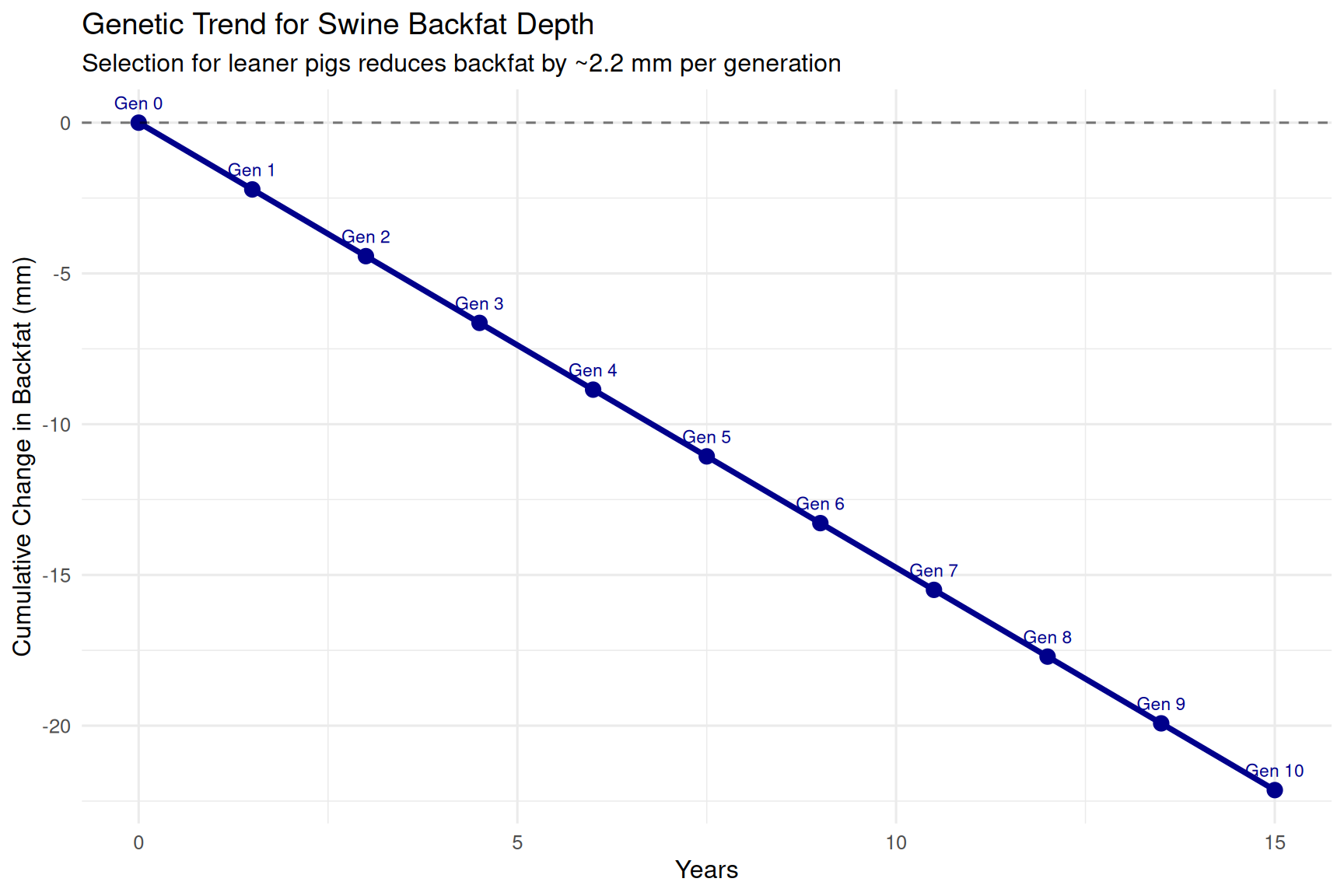
Interpretation: Over 10 generations (15 years), the breeding program reduces backfat by approximately 22.1 mm. This is a substantial genetic change, making pigs considerably leaner and improving carcass value.
6.10.3 Reality Check: Selection Response Slows Over Time
The breeder’s equation assumes that genetic parameters remain constant. In reality:
- σA decreases over time: As favorable alleles increase in frequency, genetic variation declines
- Inbreeding may increase: Reducing Ne and causing inbreeding depression
- Selection limits: Eventually, most favorable alleles are fixed, and response plateaus
These factors mean that response to selection is typically fastest in early generations and slows over time. However, for practical breeding programs (10-20 year planning horizon), the breeder’s equation remains a useful predictor.
6.10.4 Comparing Genetic Trends Across Species
Let’s visualize how genetic trends differ across our four example species:
# Create comparable genetic trend data for four species
# Standardize response as % of initial mean to make comparable

# Annual response from earlier examples
R_dairy_annual <- 222  # kg milk per year
R_swine_annual <- 0.230  # pigs per litter per year
R_broiler_annual <- 244  # grams per year
R_beef_annual <- 3.1  # kg weaning weight per year

# Initial means (approximate population averages)
mean_dairy <- 10000  # kg milk per lactation
mean_swine <- 12  # pigs per litter
mean_broiler <- 2500  # grams at 42 days
mean_beef <- 250  # kg weaning weight

# Calculate as % per year
pct_dairy <- (R_dairy_annual / mean_dairy) * 100
pct_swine <- (R_swine_annual / mean_swine) * 100
pct_broiler <- (R_broiler_annual / mean_broiler) * 100
pct_beef <- (R_beef_annual / mean_beef) * 100

# Create trend data
years_trend <- 0:20

trends_comparison <- tibble(
  Year = rep(years_trend, 4),
  Species = rep(c("Dairy (milk)", "Swine (litter size)",
                  "Broilers (body wt)", "Beef (weaning wt)"),
                each = length(years_trend)),
  Pct_per_year = rep(c(pct_dairy, pct_swine, pct_broiler, pct_beef),
                     each = length(years_trend)),
  Cumulative_Pct = Year * Pct_per_year
)

# Plot
ggplot(trends_comparison, aes(x = Year, y = Cumulative_Pct,
                               color = Species, linetype = Species)) +
  geom_line(size = 1.3) +
  geom_point(size = 2, alpha = 0.6) +
  scale_color_manual(values = c("Dairy (milk)" = "purple",
                                 "Swine (litter size)" = "red",
                                 "Broilers (body wt)" = "darkgreen",
                                 "Beef (weaning wt)" = "orange")) +
  labs(x = "Years",
       y = "Cumulative Genetic Improvement (% of base mean)",
       title = "Genetic Trends Vary Dramatically Across Species",
       subtitle = "Broilers improve fastest; swine litter size slowest (relative to trait mean)",
       color = "Species & Trait",
       linetype = "Species & Trait") +
  theme_minimal(base_size = 12) +
  theme(legend.position = c(0.25, 0.75))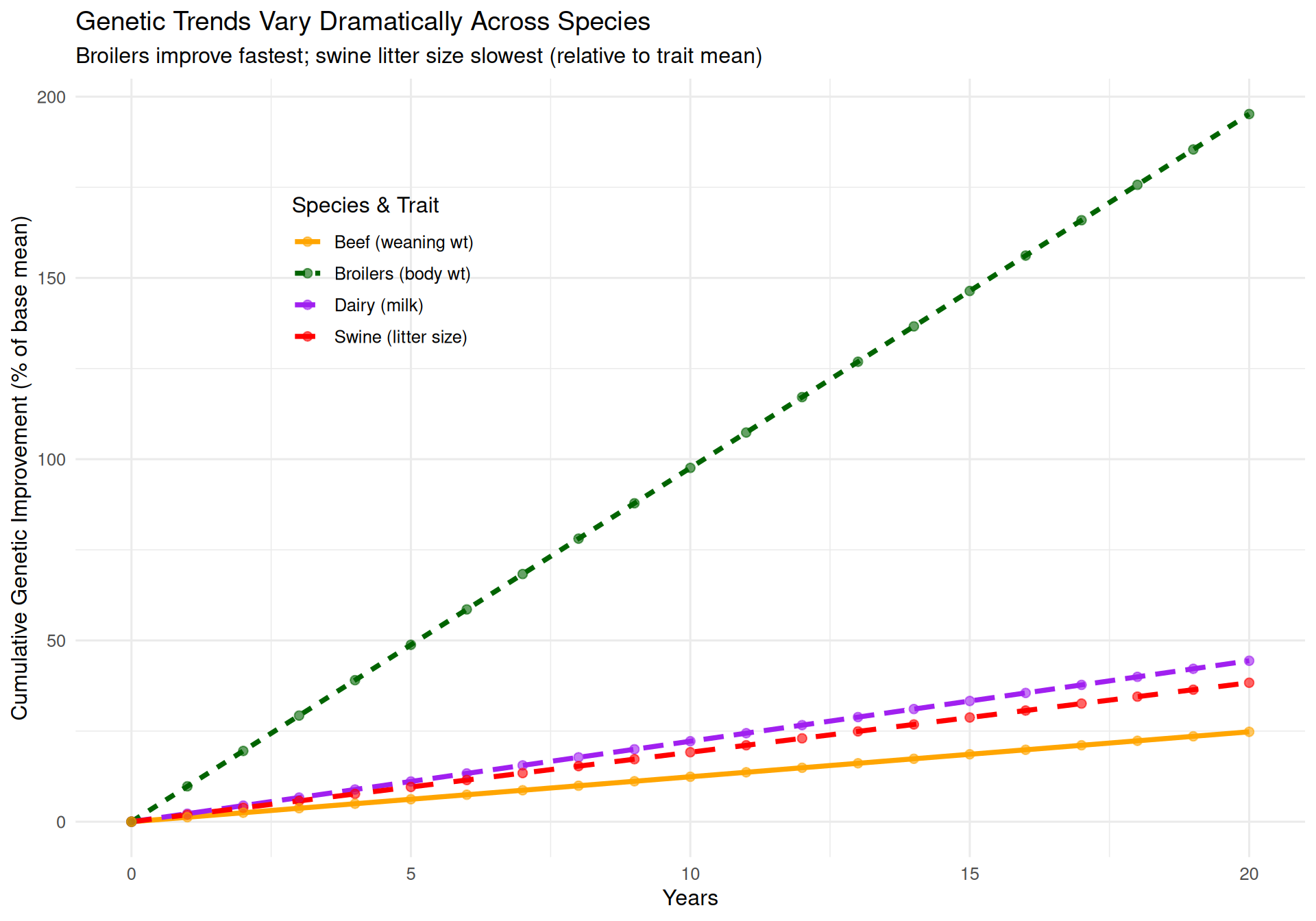
Key insights:
-
Broilers improve fastest: ~10% per year → 200% improvement over 20 years
- Short L, high i, high h²
-
Beef cattle improve slowly: ~1.2% per year → 24% improvement over 20 years
- Long L is the limiting factor
-
Swine litter size improves very slowly: ~2% per year → 40% over 20 years
- Low h² is the limiting factor
-
Dairy milk yield moderate: ~2.2% per year → 44% over 20 years
- Genomic selection dramatically improved this rate around 2009
This comparison illustrates why broiler chickens have changed so dramatically over the past 50 years, while reproductive traits in all species remain challenging to improve.
6.11 Summary
6.11.1 Key Concepts
6.11.2 Major Takeaways
Selection intensity (i): - Determined by proportion selected (p) - Higher intensity = faster progress - Limited by need for genetic diversity and reproductive capacity - Ranges from 0.8 (50% selected) to 2.67 (1% selected)
Accuracy (r): - Depends on heritability and amount of information - Progeny testing gives high accuracy (0.80-0.95) but long L - Genomic selection gives moderate accuracy (0.50-0.75) at birth - Each additional record adds less to accuracy (diminishing returns)
Genetic standard deviation (σA): - Measure of genetic variation in the population - Breeders have little control over σA - Limits ceiling for genetic improvement - Gradually decreases with selection (fixation of favorable alleles)
Generation interval (L): - Most variable factor across species (1-10 years) - Dividing by L converts per-generation to per-year response - Shortening L has been a major focus of modern breeding (genomic selection) - Trade-off with accuracy in traditional breeding
Comparing breeding strategies: - Use breeder’s equation to predict response under different scenarios - Genomic selection often optimal: balances accuracy and generation interval - Economic factors matter: cost per unit genetic gain
Multi-generation selection: - Genetic gains compound over time - Response may slow as σA decreases - Genetic trends show cumulative progress
6.11.3 Looking Forward
In Chapter 7, we’ll explore how we estimate breeding values (the basis for accuracy, r). Understanding BLUP and genomic predictions will show how we achieve the accuracies discussed in this chapter.
In Chapter 8, we’ll examine genetic correlations between traits, which complicate selection and require multi-trait selection strategies (Chapter 9).
The breeder’s equation is the foundation of all breeding program design. Mastering it enables you to predict genetic progress, compare strategies, and optimize breeding schemes for maximum genetic gain.
6.12 Practice Problems
6.12.1 Problems
Problem 1: Calculate Response to Selection
A sheep breeding program for fleece weight has the following parameters: - Selection intensity: i = 1.76 (top 10% selected) - Accuracy: r = 0.60 - Genetic standard deviation: σA = 0.59 kg - Generation interval: L = 3.0 years
Calculate: a) Response per generation b) Response per year c) Cumulative genetic gain over 15 years
Problem 2: Compare Two Selection Strategies
A poultry breeding company is choosing between two strategies for selecting for egg production:
Strategy A: Phenotypic selection - Select at 30 weeks of age based on egg production - i = 2.2, r = 0.55, σA = 11 eggs, L = 1.0 year
Strategy B: Genomic selection - Select at hatch based on GEBV - i = 2.2, r = 0.50, σA = 11 eggs, L = 0.75 years
Which strategy gives higher annual genetic gain? By how much?
Problem 3: The Accuracy-L Trade-off
A beef cattle breeder is deciding whether to progeny test bulls before widespread use. Trait: Weaning weight.
Option 1: Use bulls at 2 years without progeny test - r = 0.50 (based on own weight and pedigree) - L = 3.5 years
Option 2: Progeny test with 30 calves before widespread use - r = 0.80 (high accuracy from progeny) - L = 6.5 years (wait for calves to be born and weaned)
For both options: i = 1.8, σA = 13.4 kg
- Calculate expected annual response for each option
- Which option is better?
- What if genomic selection could achieve r = 0.65 at birth (L = 3.5 years)? Calculate response.
Problem 4: Why Does Poultry Improve So Fast?
Compare broiler body weight selection to beef weaning weight selection:
Broilers: - i = 2.6, r = 0.70, σA = 134 g, L = 1.0 year - Population mean = 2,500 g
Beef cattle: - i = 1.8, r = 0.65, σA = 13.4 kg, L = 5.0 years - Population mean = 250 kg
- Calculate annual response for both species
- Express annual response as % of population mean
- Calculate cumulative % improvement over 20 years for both
- Explain which factors contribute most to the difference
Problem 5: Optimize Selection Given Constraints
A dairy breeding program wants to maximize genetic gain for milk yield: - σA = 500 kg - Current program: i = 1.76 (10% selected), r = 0.70 (genomic), L = 3.5 years
They can make ONE of the following changes:
Option A: Increase selection intensity to i = 2.06 (5% selected) - May increase inbreeding risk - All else unchanged
Option B: Improve genomic accuracy to r = 0.80 - Requires larger reference population (costs $500K) - All else unchanged
Option C: Reduce generation interval to L = 2.8 years - Requires using younger bulls and cows - May increase facilities costs - All else unchanged
- Calculate the new R for each option
- Calculate the % improvement in R compared to current program
- Which option gives the most improvement?
- What other factors (besides R) should be considered in this decision?
6.12.2 Solutions
Problem 1 Solution:
# Given parameters
i <- 1.76
r <- 0.60
sigma_A <- 0.59
L <- 3.0

# a) Response per generation
R_per_gen <- i * r * sigma_A
cat("a) Response per generation:\n")
a) Response per generation:cat(" R = i × r × σ_A\n") R = i × r × σ_Acat(" R =", i, "×", r, "×", sigma_A, "\n") R = 1.76 × 0.6 × 0.59 R = 0.623 kg per generation# b) Response per year
R_per_year <- R_per_gen / L
cat("b) Response per year:\n")b) Response per year: R = 0.623 / 3 R = 0.208 kg per year# c) Cumulative gain over 15 years
years <- 15
cumulative_gain <- R_per_year * years
cat("c) Cumulative gain over 15 years:\n")c) Cumulative gain over 15 years: Total = 0.208 × 15 Total = 3.12 kgProblem 2 Solution:
# Strategy A: Phenotypic selection
i_A <- 2.2
r_A <- 0.55
sigma_A_A <- 11
L_A <- 1.0
R_A <- (i_A * r_A * sigma_A_A) / L_A

cat("Strategy A (Phenotypic):\n")
Strategy A (Phenotypic): R = 13.31 eggs per year# Strategy B: Genomic selection
i_B <- 2.2
r_B <- 0.50
sigma_A_B <- 11
L_B <- 0.75
R_B <- (i_B * r_B * sigma_A_B) / L_B
cat("Strategy B (Genomic):\n")Strategy B (Genomic): R = 16.13 eggs per year# Compare
difference <- R_B - R_A
pct_improvement <- (R_B / R_A - 1) * 100
cat("Comparison:\n")Comparison: Strategy B gives 2.82 more eggs per year That's a 21.2 % improvementcat("Answer: Strategy B (genomic selection) is better despite lower accuracy,\n")Answer: Strategy B (genomic selection) is better despite lower accuracy,cat(" due to shorter generation interval (0.75 vs 1.0 years)\n") due to shorter generation interval (0.75 vs 1.0 years)Problem 3 Solution:
# Common parameters
i <- 1.8
sigma_A <- 13.4

# Option 1: No progeny test
r_1 <- 0.50
L_1 <- 3.5
R_1 <- (i * r_1 * sigma_A) / L_1

cat("Option 1 (No progeny test):\n")
Option 1 (No progeny test): R = 3.45 kg per year# Option 2: Progeny test
r_2 <- 0.80
L_2 <- 6.5
R_2 <- (i * r_2 * sigma_A) / L_2
cat("Option 2 (Progeny test):\n")Option 2 (Progeny test): R = 2.97 kg per yearb) Option 1 is better ( 3.45 > 2.97 )# Option 3: Genomic selection
r_3 <- 0.65
L_3 <- 3.5
R_3 <- (i * r_3 * sigma_A) / L_3
cat("c) Genomic selection:\n")c) Genomic selection: R = 4.48 kg per yearcat("Genomic selection is the best option!\n")Genomic selection is the best option!It achieves 51 % more annual gain than progeny testingcat("by improving accuracy without increasing L.\n")by improving accuracy without increasing L.Problem 4 Solution:
# Broilers
i_broiler <- 2.6
r_broiler <- 0.70
sigma_A_broiler <- 134  # grams
L_broiler <- 1.0
mean_broiler <- 2500  # grams

R_broiler <- (i_broiler * r_broiler * sigma_A_broiler) / L_broiler

# Beef
i_beef <- 1.8
r_beef <- 0.65
sigma_A_beef <- 13.4  # kg
L_beef <- 5.0
mean_beef <- 250  # kg

R_beef <- (i_beef * r_beef * sigma_A_beef) / L_beef

cat("a) Annual response:\n")
a) Annual response: Broilers: 243.9 grams per year Beef: 3.14 kg per year# b) As % of mean
pct_broiler <- (R_broiler / mean_broiler) * 100
pct_beef <- (R_beef / mean_beef) * 100
cat("b) Annual response as % of mean:\n")b) Annual response as % of mean: Broilers: 9.76 % per year Beef: 1.25 % per year# c) Cumulative over 20 years
years <- 20
cum_pct_broiler <- pct_broiler * years
cum_pct_beef <- pct_beef * years
cat("c) Cumulative improvement over 20 years:\n")c) Cumulative improvement over 20 years: Broilers: 195 % Beef: 25 %# d) Explanation
cat("d) Factors contributing to difference:\n")d) Factors contributing to difference:cat(" 1. Generation interval: Broilers L = 1 vs Beef L = 5\n") 1. Generation interval: Broilers L = 1 vs Beef L = 5cat(" This alone accounts for a 5-fold difference!\n") This alone accounts for a 5-fold difference!cat(" 2. Selection intensity: Broilers i = 2.6 vs Beef i = 1.8\n") 2. Selection intensity: Broilers i = 2.6 vs Beef i = 1.8cat(" Broilers can select more intensely (larger populations, higher reproduction)\n") Broilers can select more intensely (larger populations, higher reproduction)cat(" 3. Accuracy: Similar (0.70 vs 0.65)\n") 3. Accuracy: Similar (0.70 vs 0.65)cat(" 4. Genetic SD: Absolute values not comparable across species\n\n") 4. Genetic SD: Absolute values not comparable across speciescat(" PRIMARY DRIVER: Generation interval (5-fold difference)\n") PRIMARY DRIVER: Generation interval (5-fold difference)cat(" SECONDARY DRIVER: Selection intensity (1.4-fold difference)\n") SECONDARY DRIVER: Selection intensity (1.4-fold difference)Problem 5 Solution:
# Current program
i_current <- 1.76
r_current <- 0.70
sigma_A <- 500
L_current <- 3.5

R_current <- (i_current * r_current * sigma_A) / L_current
cat("Current program:\n")
Current program: R = 176 kg per year# Option A: Increase intensity
i_A <- 2.06
R_A <- (i_A * r_current * sigma_A) / L_current
improvement_A <- (R_A / R_current - 1) * 100
cat("Option A (Increase intensity to i = 2.06):\n")Option A (Increase intensity to i = 2.06): R = 206 kg per year Improvement: 17 %# Option B: Improve accuracy
r_B <- 0.80
R_B <- (i_current * r_B * sigma_A) / L_current
improvement_B <- (R_B / R_current - 1) * 100
cat("Option B (Improve accuracy to r = 0.80):\n")Option B (Improve accuracy to r = 0.80): R = 201.1 kg per year Improvement: 14.3 %# Option C: Reduce L
L_C <- 2.8
R_C <- (i_current * r_current * sigma_A) / L_C
improvement_C <- (R_C / R_current - 1) * 100
cat("Option C (Reduce L to 2.8 years):\n")Option C (Reduce L to 2.8 years): R = 220 kg per year Improvement: 25 %c) Option C (reduce L) gives the most improvement: 25 %cat("d) Other factors to consider:\n")d) Other factors to consider:cat(" Option A (intensity):\n") Option A (intensity):cat(" - May increase inbreeding and reduce genetic diversity\n") - May increase inbreeding and reduce genetic diversitycat(" - Need to monitor inbreeding coefficient\n") - Need to monitor inbreeding coefficientcat(" - Could implement OCS to manage inbreeding\n\n") - Could implement OCS to manage inbreedingcat(" Option B (accuracy):\n") Option B (accuracy):cat(" - Requires $500K investment in reference population\n") - Requires $500K investment in reference populationcat(" - Calculate cost per kg genetic gain\n") - Calculate cost per kg genetic gaincat(" - One-time investment with ongoing benefits\n\n") - One-time investment with ongoing benefitscat(" Option C (reduce L):\n") Option C (reduce L):cat(" - Requires facilities for younger animals\n") - Requires facilities for younger animalscat(" - May have lower production from younger cows\n") - May have lower production from younger cowscat(" - Consider economic returns from shorter L\n\n") - Consider economic returns from shorter Lcat(" RECOMMENDATION: Option C gives best genetic gain,\n") RECOMMENDATION: Option C gives best genetic gain,cat(" but conduct full economic analysis including facility costs\n") but conduct full economic analysis including facility costscat(" and production losses from using younger animals.\n") and production losses from using younger animals.6.13 Further Reading
6.13.1 Classic Textbooks
Falconer, D.S. and Mackay, T.F.C. Introduction to Quantitative Genetics (4th edition). Longman, 1996. - Chapter 11: Selection—basic theory and breeder’s equation derivation - Chapter 13: Selection—advanced topics including correlated response
Lynch, M. and Walsh, B. Genetics and Analysis of Quantitative Traits. Sinauer Associates, 1998. - Chapter 12: Selection on a single trait - Chapter 13: Measuring selection - Comprehensive mathematical treatment
Bourdon, R.M. Understanding Animal Breeding (2nd edition). Prentice Hall, 2000. - Very accessible introduction to breeder’s equation - Practical examples from livestock breeding
6.13.2 Historical Papers
Lush, J.L. (1945). Animal Breeding Plans (3rd edition). Iowa State College Press. - Foundational book that formalized the breeder’s equation - Historical perspective on early animal breeding
Rendel, J.M. and Robertson, A. (1950). Estimation of genetic gain in milk yield by selection in a closed herd of dairy cattle. Journal of Genetics 50: 1-8. - Classic paper demonstrating prediction and realization of selection response
6.13.3 Genomic Selection Impact
Hayes, B.J., Bowman, P.J., Chamberlain, A.J., and Goddard, M.E. (2009). Invited review: Genomic selection in dairy cattle—Progress and challenges. Journal of Dairy Science 92: 433-443. - Overview of how genomic selection changed dairy breeding
García-Ruiz, A., Cole, J.B., VanRaden, P.M., Wiggans, G.R., Ruiz-López, F.J., and Van Tassell, C.P. (2016). Changes in genetic selection differentials and generation intervals in US Holstein dairy cattle as a result of genomic selection. PNAS 113: E3995-E4004. - Quantifies how genomic selection reduced generation intervals and increased gain
Schaeffer, L.R. (2006). Strategy for applying genome-wide selection in dairy cattle. Journal of Animal Breeding and Genetics 123: 218-223. - Early proposal for implementing genomic selection
6.13.4 Trade-offs and Breeding Program Design
Bijma, P. (2012). Accuracies of estimated breeding values from ordinary genetic evaluations do not reflect the correlation between true and estimated breeding values in selected populations. Journal of Animal Breeding and Genetics 129: 345-358. - Discussion of accuracy in selection programs
Woolliams, J.A., Berg, P., Dagnachew, B.S., and Meuwissen, T.H.E. (2015). Genetic contributions and their optimization. Journal of Animal Breeding and Genetics 132: 89-99. - Optimizing contributions to balance gain and inbreeding
6.13.5 Online Resources
Beef Improvement Federation (BIF) Guidelines - https://beefimprovement.org/ - Practical application of selection theory to beef cattle
Council on Dairy Cattle Breeding (CDCB) - https://uscdcb.com/ - Genetic evaluations, trends, and documentation
National Swine Improvement Federation - Guidelines for genetic evaluation in swine - Practical breeding program design