| Species | Trait | Units | σ²_P | σ²_A | σ²_E | h² |
|---|---|---|---|---|---|---|
| Swine | ||||||
| Swine | Backfat depth | mm² | 9.00e+00 | 5.40e+00 | 3.60e+00 | 0.60 |
| Swine | Average daily gain | g²/day² | 2.50e+03 | 1.25e+03 | 1.25e+03 | 0.50 |
| Swine | Feed conversion ratio | (kg/kg)² | 4.00e-02 | 1.00e-02 | 3.00e-02 | 0.30 |
| Swine | Litter size (NBA) | piglets² | 6.25e+00 | 7.50e-01 | 5.50e+00 | 0.12 |
| Swine | Loin depth | mm² | 1.60e+01 | 8.00e+00 | 8.00e+00 | 0.50 |
| Dairy Cattle | ||||||
| Dairy | Milk yield (305-d) | kg² | 9.00e+05 | 2.70e+05 | 6.30e+05 | 0.30 |
| Dairy | Fat percentage | %² | 2.50e-01 | 1.30e-01 | 1.20e-01 | 0.52 |
| Dairy | Protein percentage | %² | 1.20e-01 | 6.00e-02 | 6.00e-02 | 0.50 |
| Dairy | Somatic cell score | score² | 2.25e+00 | 2.70e-01 | 1.98e+00 | 0.12 |
| Dairy | Daughter pregnancy rate | %² | 2.50e+01 | 2.50e+00 | 2.25e+01 | 0.10 |
| Beef Cattle | ||||||
| Beef | Weaning weight | kg² | 6.25e+02 | 2.81e+02 | 3.44e+02 | 0.45 |
| Beef | Yearling weight | kg² | 1.60e+03 | 8.00e+02 | 8.00e+02 | 0.50 |
| Beef | Marbling score | score² | 6.40e-01 | 2.60e-01 | 3.80e-01 | 0.40 |
| Beef | Ribeye area | cm⁴ | 3.60e+01 | 1.62e+01 | 1.98e+01 | 0.45 |
| Broilers | ||||||
| Broiler | Body weight (42-d) | g² | 1.00e+04 | 3.50e+03 | 6.50e+03 | 0.35 |
| Broiler | Feed efficiency | g² | 4.00e+02 | 1.60e+02 | 2.40e+02 | 0.40 |
| Broiler | Breast yield | %² | 4.00e+00 | 2.00e+00 | 2.00e+00 | 0.50 |
| Layers | ||||||
| Layer | Egg production (to 72 wk) | eggs² | 4.00e+02 | 1.00e+02 | 3.00e+02 | 0.25 |
| Layer | Egg weight | g² | 9.00e+00 | 4.50e+00 | 4.50e+00 | 0.50 |
| Layer | Shell strength | N² | 1.60e+01 | 6.40e+00 | 9.60e+00 | 0.40 |
| Sheep | ||||||
| Sheep | Weaning weight | kg² | 1.60e+01 | 6.40e+00 | 9.60e+00 | 0.40 |
| Sheep | Fleece weight | kg² | 1.00e+00 | 5.00e-01 | 5.00e-01 | 0.50 |
| Sheep | Litter size | lambs² | 3.60e-01 | 4.00e-02 | 3.20e-01 | 0.11 |
3 The Basic Genetic Model
Learning Objectives
By the end of this chapter, you will be able to:
- Partition a phenotype into genetic and environmental components
- Distinguish between additive, dominance, and epistatic genetic effects
- Explain why additive effects are the primary focus of animal breeding
- Understand the concept of variance partitioning
- Calculate breeding values from a simple genetic model
3.1 Introduction
Imagine you’re visiting a commercial swine operation, standing in front of a finishing pen with 20 pigs that are all about 20 weeks old. You notice something immediately: these pigs aren’t all the same size. Some weigh 100 kg, others weigh 115 kg, and a few are pushing 125 kg. This variation raises a fundamental question that has driven animal breeding for centuries:
Why are these animals different from each other?
More specifically: Are the heavier pigs genetically superior, or did they just have better luck—better health, better access to feeders, or better pen mates that didn’t compete as aggressively for feed? If you’re selecting which animals to keep as breeding stock, this question isn’t just academic—it’s worth millions of dollars to a breeding company. Choose the wrong animals (those with good environments but poor genetics), and you’ll make little genetic progress. Choose the right ones (those with genuinely superior genetics), and you’ll steadily improve the herd, generation after generation.
The challenge is that we can only observe the phenotype—the animal’s actual weight, milk production, or growth rate. But what we really care about for breeding purposes is the animal’s genetic merit—the portion of its performance that will be transmitted to its offspring. We need a way to separate these two components.
In Chapter 2, we discussed how to measure phenotypes accurately and why high-quality data collection is essential. We introduced the concept of True Breeding Value (TBV)—an animal’s true genetic merit that determines what it passes to its offspring. But we didn’t yet address how phenotypes and breeding values relate to each other mathematically. That’s the purpose of this chapter.
3.1.1 The Fundamental Genetic Model
The key insight that makes modern animal breeding possible is surprisingly simple: we can think of an animal’s phenotype as the sum of two components:
- Genetic effects: What the animal inherited from its parents
- Environmental effects: Everything else (nutrition, health, management, luck)
Mathematically, we express this as:
\[ y = \mu + A + E \]
This equation—arguably the most important equation in all of animal breeding—says that an animal’s phenotype (\(y\)) equals the population mean (\(\mu\)) plus its genetic merit (\(A\), the additive genetic effect or breeding value) plus environmental influences (\(E\)).
While this model looks simple, it has profound implications:
- It explains why animals with the same genetics can have different phenotypes (different environments)
- It explains why animals with the same phenotype can have different genetics (environment compensates or masks genetic differences)
- It provides a framework for estimating breeding values from phenotypic data
- It allows us to predict response to selection based on how much genetic variance exists in the population
3.1.2 Not All Genetic Effects Are Equal
Here’s where it gets more interesting: “genetic effects” aren’t a single, monolithic thing. When we look closely, we find that genetic effects can be partitioned into three types:
- Additive effects (\(A\)): The effects that breed true and pass predictably from parent to offspring—these determine breeding value
- Dominance effects (\(D\)): Within-locus interactions between alleles that don’t transmit reliably
- Epistatic effects (\(I\)): Between-locus interactions that are even more complex and unpredictable
The remarkable discovery that revolutionized animal breeding in the mid-20th century is that only additive effects matter for long-term genetic improvement. Dominance and epistasis can affect an individual animal’s performance, but they don’t breed true. When you select parents based on their phenotypes, only the additive portion of their genetic merit reliably appears in their offspring.
This is why we focus breeding programs on estimating and selecting for additive genetic effects—what we call breeding values. A bull with a high breeding value for milk production will tend to have daughters that produce a lot of milk, regardless of what dominance or epistatic effects happened to make the bull himself a high or low producer.
3.1.3 What You’ll Learn in This Chapter
In this chapter, we’ll build a complete understanding of the basic genetic model that underlies all of quantitative genetics and animal breeding. Specifically, we’ll:
- Define the model \(y = \mu + A + E\) and understand what each component represents
- Explore the three types of genetic effects (additive, dominance, epistatic) and understand why they differ in importance
- Learn why additive effects are the primary focus of animal breeding programs
- Partition variance into genetic and environmental components, setting up the concept of heritability (Chapter 5)
- Work through numerical examples for multiple livestock species, showing how the model applies to real breeding scenarios
- Understand parent-offspring relationships and why offspring resemble their parents (but not perfectly)
- Simulate the model in R to visualize how genetic and environmental effects combine to create observed phenotypes
This chapter lays the foundation for everything that follows. Understanding how to partition phenotypes into genetic and environmental components is essential for:
- Estimating heritability (Chapter 5)
- Predicting response to selection (Chapter 6)
- Understanding genetic correlations between traits (Chapter 8)
- Estimating breeding values with BLUP (Chapter 7)
- Appreciating why genomic selection works (Chapter 13)
Think of this chapter as learning the grammar of the language of quantitative genetics. Once you understand the basic model, the more complex topics in later chapters will make much more sense because they’re all extensions or applications of these fundamental ideas.
A Note on Terminology
You’ll encounter several related terms in this chapter and throughout the book:
- Breeding value (BV) = Additive genetic effect (\(A\)) = Sum of additive effects of all an animal’s alleles
- True breeding value (TBV) = An animal’s actual, unknown breeding value (what we’re trying to estimate)
- Estimated breeding value (EBV) = Our statistical prediction of an animal’s TBV (covered in Chapter 7)
These terms are often used interchangeably in practice, but the distinctions matter: TBV is the truth (unknown), EBV is our estimate (known but imperfect), and BV is the general concept.
Let’s start by carefully defining each component of the basic genetic model.
3.2 The Basic Model: y = μ + A + E
At its heart, the basic genetic model describes how an individual animal’s observed performance (phenotype) is determined by the combination of its genetic merit and the environment it experienced. Let’s build this model carefully, starting with the conceptual idea and then moving to the mathematical representation.
3.2.1 Conceptual Framework
Think of an animal’s phenotype as the outcome of a “recipe” with three ingredients:
- The species baseline: What’s typical for the population (e.g., the average weaning weight for pigs in this herd)
- The animal’s unique genetics: Whether this particular animal inherited genes that make it grow faster or slower than average
- The animal’s unique experiences: Whether it had good nutrition, stayed healthy, competed successfully for feed, etc.
These three components combine additively—they simply add together to produce the final phenotype. This is expressed mathematically as:
\[ y = \mu + A + E \]
This equation is deceptively simple, but it encapsulates a profound insight: phenotype is the sum of nature (genetics) and nurture (environment). Let’s define each component precisely.
3.2.2 Components of the Model
Let’s be very clear about what these components represent:
\(y\) is observable: We can weigh the pig, milk test the cow, or record the racing time. This is our data.
\(\mu\) is estimable: We can calculate the mean of all observations in a contemporary group (animals managed similarly).
\(A\) is NOT directly observable: We cannot open up an animal and “see” its breeding value. This is the challenge of animal breeding—we must estimate \(A\) from phenotypic data and pedigree/genomic information (Chapter 7).
\(E\) is NOT directly observable: For any individual animal, we can’t know exactly what environmental advantages or disadvantages it experienced.
However, once we know \(y\) and \(\mu\), we can calculate the phenotypic deviation:
\[ (y - \mu) = A + E \]
The animal’s deviation from the population mean is due to the sum of its genetic merit and environmental effects. Our challenge as breeders is to separate these two components—to figure out how much of \((y - \mu)\) is due to \(A\) (good genetics) versus \(E\) (good environment).
3.2.3 Why This Model Matters
This simple model is the foundation of all modern animal breeding. Here’s why it’s so powerful:
1. It explains variation between animals
Why is Pig #347 heavier than Pig #251? Three possibilities: - Pig #347 has better genetics (\(A_{347} > A_{251}\)) - Pig #347 had a better environment (\(E_{347} > E_{251}\)) - Some combination of both
2. It provides a framework for estimating breeding values
If we can account for environmental effects (e.g., by comparing animals in the same pen, born in the same season), we can make informed guesses about their genetic merit. This is the basis for BLUP (Best Linear Unbiased Prediction) in Chapter 7.
3. It connects to response to selection
When we select parents based on their phenotypes, the genetic progress we make depends on how accurately we’ve estimated \(A\). If phenotypic differences are mostly genetic (\(A\) is large relative to \(E\)), selection is effective. If differences are mostly environmental (\(E\) dominates), selection is less effective. This connects directly to heritability (Chapter 5).
4. It generalizes to complex scenarios
This basic model can be extended to handle multiple traits, repeated measurements, maternal effects, and genomic information—but the core structure remains \(y = \mu + A + E\).
3.2.4 Example 1: Weaning Weight in Swine
Let’s work through a concrete numerical example to make this model tangible. Consider weaning weight (measured at 21 days of age) in a population of piglets.
Population parameters: - \(\mu = 6.0\) kg (population mean weaning weight) - Typical range: 4.5 to 7.5 kg
Now let’s look at three specific piglets and decompose their phenotypes:
Piglet #1 (Heavy piglet) - Phenotype: \(y_1 = 7.1\) kg - Breeding value: \(A_1 = +0.8\) kg (genetically superior; 0.8 kg above average) - Environmental effect: \(E_1 = +0.3\) kg (slightly favorable environment) - Check: \(y_1 = 6.0 + 0.8 + 0.3 = 7.1\) kg ✓
This piglet is heavy (7.1 kg vs. mean of 6.0 kg) for two reasons: it has good genetics (+0.8 kg) and it had a slightly advantageous environment (+0.3 kg). Perhaps it had better access to the sow’s teats, or it avoided early disease.
Piglet #2 (Above-average piglet) - Phenotype: \(y_2 = 6.4\) kg - Breeding value: \(A_2 = -0.5\) kg (genetically inferior; 0.5 kg below average) - Environmental effect: \(E_2 = +0.9\) kg (very favorable environment) - Check: \(y_2 = 6.0 - 0.5 + 0.9 = 6.4\) kg ✓
This piglet is above average phenotypically (6.4 kg vs. 6.0 kg), but it’s not genetically superior. In fact, it has below-average genetics (\(A = -0.5\) kg). Its above-average performance is entirely due to a very favorable environment (+0.9 kg). If we selected this animal as a parent based on phenotype alone, we’d be disappointed—its offspring would inherit the poor genetics, not the lucky environment.
Piglet #3 (Light piglet) - Phenotype: \(y_3 = 5.5\) kg - Breeding value: \(A_3 = +0.2\) kg (genetically slightly above average!) - Environmental effect: \(E_3 = -0.7\) kg (unfavorable environment) - Check: \(y_3 = 6.0 + 0.2 - 0.7 = 5.5\) kg ✓
This piglet appears inferior phenotypically (5.5 kg, well below the mean). But here’s the surprising insight: it actually has positive genetic merit (\(A = +0.2\) kg). It’s light because it experienced a poor environment (−0.7 kg)—maybe it got sick, or was outcompeted by littermates. If we cull this animal based on phenotype alone, we’re discarding positive genetic merit.
The Central Challenge of Animal Breeding
We can observe \(y\), but we need to know \(A\).
Piglet #2 (y = 6.4 kg, A = −0.5 kg) looks better than Piglet #3 (y = 5.5 kg, A = +0.2 kg), but Piglet #3 is genetically superior. This example illustrates why animal breeding is not just about selecting animals with high phenotypes—it’s about estimating breeding values and selecting animals with high genetic merit, regardless of their environmental luck.
The better we can estimate \(A\) from observable data (\(y\), pedigree, genomics), the more genetic progress we make. This is why methods like BLUP (Chapter 7) and genomic selection (Chapter 13) are so valuable—they help us “see through” the environmental noise to the underlying genetic signal.
3.2.5 Example 2: Milk Yield in Dairy Cattle
Let’s look at another species to reinforce the concept. Consider 305-day mature-equivalent milk yield in Holstein dairy cattle.
Population parameters: - \(\mu = 10,000\) kg (population mean) - Typical range: 7,000 to 13,000 kg
Cow #2417 - Phenotype: \(y = 11,500\) kg (high-producing cow) - Breeding value: \(A = +1,200\) kg (genetically superior) - Environmental effect: \(E = +300\) kg (good management) - Check: \(y = 10,000 + 1,200 + 300 = 11,500\) kg ✓
This cow is an excellent producer, and she’s genetically superior (+1,200 kg breeding value). If we use her as a dam, her daughters will inherit, on average, half of her breeding value (more on this in Section 3.7). We’d expect her daughters to have breeding values around \(+1,200/2 = +600\) kg, making them well above average.
Cow #1853 - Phenotype: \(y = 11,200\) kg (also high-producing) - Breeding value: \(A = +400\) kg (modestly above average) - Environmental effect: \(E = +800\) kg (exceptional management) - Check: \(y = 10,000 + 400 + 800 = 11,200\) kg ✓
This cow has a similar phenotype to Cow #2417 (11,200 vs. 11,500 kg), but she’s much less genetically valuable. Most of her high production is due to excellent management—perhaps she was in a herd with superior feeding, or she avoided health problems. If we breed her, her daughters will only inherit the +400 kg genetic component, not the +800 kg environmental advantage.
Cow #3692 - Phenotype: \(y = 9,100\) kg (below average) - Breeding value: \(A = +600\) kg (actually above average genetically!) - Environmental effect: \(E = -1,500\) kg (serious health or management problems) - Check: \(y = 10,000 + 600 - 1,500 = 9,100\) kg ✓
This cow produced only 9,100 kg—well below the herd average. A naive breeder might cull her. But she has positive genetic merit (+600 kg)! Her low production was due to severe environmental challenges (−1,500 kg)—perhaps she had mastitis, lameness, or poor nutrition. If we can identify her positive genetics (through pedigree information, progeny records, or genomic testing), she could be a valuable dam.
3.2.6 Sources of Environmental Variation (\(E\))
What exactly constitutes “environmental” effects? The \(E\) term is a catch-all for everything that’s not additive genetic. Major sources include:
Nutrition and management - Feed quality and quantity - Housing conditions (temperature, humidity, space) - Milking frequency (dairy) - Pen mates and social stress
Health - Infectious disease exposure - Parasite load - Immune status - Injury or lameness
Microenvironment - Birth order and colostrum intake - Maternal effects (quality of dam, not inherited by animal itself) - Random developmental variation (stochastic biological processes)
Measurement error - Scale calibration errors - Timing of measurement (e.g., dairy test day vs. full lactation) - Observer variation in subjective scores
Age, parity, and season - Age at measurement (growing animals) - Lactation number (dairy cows produce more in later parities) - Season of birth (temperature, photoperiod, disease pressure)
In practice, we try to account for known environmental effects by using statistical models. For example:
- Contemporary groups: Compare animals born in the same season, on the same farm, in the same pen
- Fixed effects in BLUP: Adjust for known environmental factors like age, sex, parity
- Environmental covariates: Include feed intake, temperature, or other measurements in the model
After accounting for these known effects, what remains in \(E\) is random, unpredictable variation—the “luck” each animal experienced.
Common Misconception: “Genetic vs. Environmental”
Students often misinterpret the model \(y = \mu + A + E\) as saying that genetics and environment are competing forces, or that a trait can be “mostly genetic” or “mostly environmental.” This is a fundamental misunderstanding.
Correct interpretation: The model describes how genetics (\(A\)) and environment (\(E\)) both contribute to the phenotype. The question is not “Is this trait genetic or environmental?” but rather “How much of the variation in this trait across the population is due to genetic differences vs. environmental differences?”
- All traits are influenced by both genes and environment
- The relative importance of \(A\) vs. \(E\) determines heritability (Chapter 5)
- High heritability doesn’t mean environment is unimportant—it means genetic differences explain most of the variation in the population
For example, body weight in pigs is clearly influenced by both genetics (some pigs have genes for rapid growth) and environment (well-fed pigs grow faster). The model quantifies the relative contribution of each to explaining why pigs differ from each other.
3.2.7 Assumptions of the Basic Model
Before we move on, let’s state the assumptions underlying this simple model:
Additivity: The genetic and environmental effects simply add together. There’s no interaction (genotype-by-environment interaction) where certain genotypes perform better in certain environments. (We’ll relax this assumption in advanced models.)
Independence: \(A\) and \(E\) are uncorrelated. The genetic merit of an animal doesn’t affect what environment it experiences. (This can be violated if we preferentially feed high-producing animals, creating covariance between \(A\) and \(E\).)
Normally distributed effects: Both \(A\) and \(E\) follow normal distributions in the population. This assumption is reasonable for most quantitative traits and makes the math tractable.
Single environment: We’re assuming all animals are raised in reasonably similar environments that can be described by a single \(E\) term. If animals are raised in very different environments (e.g., grazing vs. confinement), we need more complex models with multiple environmental effects.
These assumptions are simplifications, but they work remarkably well for most practical breeding applications. As we progress through the book, we’ll see how to extend the model when these assumptions are violated.
3.2.8 Summary of the Basic Model
The equation \(y = \mu + A + E\) is elegant in its simplicity, yet powerful in its implications:
- Phenotypes (\(y\)) are observable; they’re what we measure
- Population mean (\(\mu\)) is the baseline, estimable from data
- Breeding values (\(A\)) are the genetic merit we care about, but they’re hidden—we must estimate them
- Environmental effects (\(E\)) are everything else, also hidden
The fundamental challenge of animal breeding is to separate \(A\) from \(E\) so we can identify and select animals with superior genetic merit. The rest of this book is essentially about solving this challenge using progressively more sophisticated methods.
In the next section, we’ll dive deeper into the genetic component (\(A\)), exploring how it can be further partitioned into additive, dominance, and epistatic effects—and why only the additive portion matters for breeding.
3.3 Types of Genetic Effects
So far, we’ve treated the genetic component of the model (\(A\)) as a single entity. But when we look more closely at how genes affect phenotypes, we discover that genetic effects can be partitioned into three fundamentally different types. Understanding these distinctions is critical because only one type—additive effects—determines what parents pass to their offspring.
The complete genetic value of an individual can be written as:
\[ G = A + D + I \]
Where: - \(G\) = Genotypic value (total genetic effect on phenotype) - \(A\) = Additive genetic effect (breeding value) - \(D\) = Dominance deviation (within-locus interaction) - \(I\) = Epistatic deviation (between-locus interaction)
For most practical breeding applications, we simplify the model by lumping \(D\) and \(I\) into the environmental term (\(E\)), giving us the basic model \(y = \mu + A + E\). But to understand why we focus on \(A\), we need to understand what \(D\) and \(I\) represent and why they don’t breed true.
3.3.1 Additive Genetic Effects (\(A\))
Definition: The additive genetic effect is the sum of the average effects of all alleles that an individual carries across all loci. It represents the portion of genetic value that is transmitted predictably from parent to offspring.
Conceptual Understanding
Think of each allele as contributing a certain “dose” of effect to the phenotype, and these doses add up linearly:
- If an animal inherits an allele that adds +2 kg to body weight, it gets +2 kg
- If it inherits two such alleles (homozygous), it gets +4 kg
- If it inherits one +2 kg allele and one −1 kg allele, it gets +1 kg total
The key property of additive effects is linearity: the effect of having two copies of an allele is exactly twice the effect of having one copy.
Simple Single-Locus Example
Consider a single gene affecting weaning weight in pigs with two alleles: - Allele \(B\) (beneficial): average effect of +1.0 kg - Allele \(b\) (less beneficial): average effect of −1.0 kg
The three possible genotypes and their additive genetic values:
| Genotype | Additive Value | Interpretation |
|---|---|---|
| \(BB\) | +2.0 kg | Two copies of beneficial allele |
| \(Bb\) | 0.0 kg | One beneficial, one less beneficial (average) |
| \(bb\) | −2.0 kg | Two copies of less beneficial allele |
Notice the perfect linearity: the heterozygote (\(Bb\)) has exactly the average of the two homozygotes: \((+2.0 + (-2.0)) / 2 = 0.0\) kg.
Reality: Polygenic Traits
In practice, economically important traits in livestock are affected by thousands of genes, each with small additive effects. An animal’s breeding value is the sum of effects across all these loci:
\[ A = \sum_{i=1}^{n} a_i \]
Where \(a_i\) is the additive effect at locus \(i\), and \(n\) is the total number of loci (typically thousands to tens of thousands for complex traits like growth rate or milk production).
This is why quantitative traits show continuous variation rather than discrete categories—the combined effect of many genes creates a smooth distribution of phenotypes.
Why Additive Effects Breed True
Here’s the crucial insight: when an animal passes one of its two alleles at each locus to its offspring, the offspring inherits half of the parent’s additive genetic value, on average:
\[ E(A_{offspring}) = \frac{1}{2}A_{sire} + \frac{1}{2}A_{dam} \]
(Plus a deviation due to Mendelian sampling—the random sampling of parental alleles—covered in Section 3.7.)
This predictability is what makes selection work: if we choose parents with high breeding values, their offspring will tend to have high breeding values too.
3.3.2 Dominance Effects (\(D\))
Definition: Dominance is a within-locus interaction where the heterozygote’s value differs from the average of the two homozygotes. Dominance effects represent deviations from additivity at individual genes.
Conceptual Understanding
Dominance occurs when alleles at the same locus interact such that having two different alleles (heterozygote) produces a phenotype that’s not exactly intermediate between the two homozygotes.
There are several types of dominance:
- Complete dominance: The heterozygote resembles one homozygote entirely
- Partial dominance: The heterozygote is closer to one homozygote but not identical
- Overdominance (rare): The heterozygote exceeds both homozygotes
Single-Locus Example with Dominance
Let’s revisit the same gene affecting weaning weight, but now with dominance:
- Allele \(B\): beneficial
- Allele \(b\): less beneficial
- Dominance: \(B\) is partially dominant over \(b\)
| Genotype | Genotypic Value | Additive Component | Dominance Deviation |
|---|---|---|---|
| \(BB\) | +2.5 kg | +2.0 kg | +0.5 kg |
| \(Bb\) | +1.5 kg | 0.0 kg | +1.5 kg |
| \(bb\) | −2.0 kg | −2.0 kg | 0.0 kg |
Notice that: - The additive component is the same as before (perfectly linear) - The dominance deviation captures how much each genotype deviates from additive expectation - The heterozygote \(Bb\) has a genotypic value (+1.5 kg) that’s better than the additive prediction (0.0 kg), thanks to dominance (+1.5 kg)
If we set \(bb\) as the reference (genotypic value = 0): - The average effect of substituting \(b\) with \(B\) is +2.25 kg (this determines the additive value) - But the heterozygote \(Bb\) gets a +1.5 kg “bonus” from dominance
Why Dominance Doesn’t Breed True
Here’s the problem: dominance effects don’t transmit predictably to offspring. Let’s see why.
Consider a \(Bb\) heterozygote pig with: - Additive value: \(A = 0.0\) kg (average of \(BB\) and \(bb\)) - Dominance deviation: \(D = +1.5\) kg - Genotypic value: \(G = +1.5\) kg (phenotypically superior)
This pig has a good phenotype (genotypic value of +1.5 kg) thanks to dominance. But when it reproduces:
- It passes either \(B\) or \(b\) to each offspring (50% chance each)
- Offspring can be \(BB\), \(Bb\), or \(bb\) depending on the other parent
- The dominance effect (+1.5 kg) only occurs in \(Bb\) offspring, not in \(BB\) or \(bb\) offspring
If this \(Bb\) pig is mated to a \(bb\) pig: - 50% of offspring are \(Bb\) (genotypic value +1.5 kg) - 50% of offspring are \(bb\) (genotypic value −2.0 kg) - Average offspring genotypic value: \((+1.5 + (-2.0)) / 2 = -0.25\) kg
The parent had a genotypic value of +1.5 kg, but the offspring average only −0.25 kg. The dominance effect was “lost” in the offspring that didn’t receive the \(Bb\) genotype.
Key insight: Dominance is a property of the genotype (the combination of alleles), not the individual alleles. When alleles are passed to offspring and recombined with alleles from the other parent, the specific genotype (and its dominance effect) is not preserved.
Dominance in Practical Breeding
For purebred (within-line) selection, dominance effects are essentially noise—they make some animals phenotypically better or worse, but they don’t transmit predictably. We can’t select for dominance directly; it gets “shuffled” each generation during reproduction.
However, dominance plays a crucial role in crossbreeding (Chapter 11). When we mate animals from two different breeds or lines, the crossbred offspring are heterozygous at many loci, and dominance effects across the genome combine to create heterosis (hybrid vigor). This is why crossbreeding is so effective for traits with low heritability, like reproduction and survival—traits where dominance effects are substantial.
3.3.3 Epistatic Effects (\(I\))
Definition: Epistasis refers to between-locus interactions where the effect of an allele at one gene depends on which alleles are present at other genes. Epistatic effects represent deviations from additivity across multiple genes.
Conceptual Understanding
While dominance is about how alleles interact within a locus, epistasis is about how alleles interact between loci. The phenotypic effect of a genotype at Gene A might depend on the genotype at Gene B.
Examples of epistasis: - Complementary gene action: Two genes must both be “active” for a trait to be expressed - Suppressor genes: An allele at one locus masks the effect of alleles at another locus - Modifier genes: An allele at one locus enhances or diminishes the effect of another locus
Example: Two-Locus Epistasis
Consider two genes affecting muscle growth in beef cattle:
-
Gene 1 (Myostatin): Determines baseline muscle development
- \(M\) (normal), \(m\) (enhanced muscle)
-
Gene 2 (IGF-1, Insulin-like Growth Factor): Modifies the effect of Myostatin
- \(I\) (high IGF), \(i\) (low IGF)
Without epistasis, we’d expect the effects to add independently. With epistasis, the effect of having \(mm\) (myostatin mutation, double muscling) depends on the IGF-1 genotype:
| Genotype at Gene 1 | Genotype at Gene 2 | Expected (Additive) | Observed (With Epistasis) | Epistatic Deviation |
|---|---|---|---|---|
| \(MM\) | \(II\) | 0 kg | 0 kg | 0 kg |
| \(MM\) | \(Ii\) | −1 kg | −0.8 kg | +0.2 kg |
| \(mm\) | \(II\) | +8 kg | +6 kg | −2 kg |
| \(mm\) | \(Ii\) | +7 kg | +10 kg | +3 kg |
In this hypothetical example, the \(mm\) genotype (double muscling) provides a much larger benefit when combined with the heterozygous \(Ii\) genotype at IGF-1, due to a synergistic interaction between the two genes. This is epistasis: the effect of \(mm\) depends on the genetic background at Gene 2.
Why Epistasis Doesn’t Breed True
Like dominance, epistasis depends on specific combinations of genotypes across multiple loci. When parents reproduce, their alleles are shuffled and recombined, breaking apart favorable (or unfavorable) epistatic combinations.
Consider a bull with genotype \(mmIi\) that has exceptional muscle growth (+10 kg) due to the favorable epistatic interaction. When he reproduces:
- He passes either \(m\) or \(I\)/\(i\) to offspring
- Offspring receive other alleles from the dam
- The specific combination \(mmIi\) may not be recreated in offspring
- Epistatic effects are not reliably transmitted
With thousands of loci involved in quantitative traits, the number of possible epistatic interactions is astronomical (pairwise interactions alone: \(n(n-1)/2\) where \(n\) is the number of loci). These interactions are constantly reshuffled during reproduction, making them unpredictable and non-heritable in any simple sense.
Epistasis in Practical Breeding
Like dominance, epistasis affects individual phenotypes but doesn’t contribute to predictable response to selection. In practical breeding programs:
- For purebred selection, we largely ignore epistasis—it’s absorbed into the environmental term or treated as random noise
- For crossbreeding, epistasis (along with dominance) may contribute to heterosis, though dominance is thought to be the primary mechanism
- In genomic selection (Chapter 13), some epistatic effects may be captured implicitly if favorable combinations happen to be in linkage disequilibrium with markers
Some cutting-edge research explores explicitly modeling epistatic interactions using genomic data, but this is computationally challenging and not yet standard practice in livestock breeding.
3.3.4 Genotypic Value vs. Breeding Value: A Crucial Distinction
Let’s solidify the difference between an animal’s genotypic value (total genetic effect on its own phenotype) and its breeding value (what it transmits to offspring):
Genotypic Value (\(G\)): \[ G = A + D + I \]
This is the animal’s total genetic contribution to its own phenotype. It includes additive effects (breed true), dominance effects (specific to this individual’s genotype), and epistatic effects (specific to this individual’s combination of genotypes across loci).
Breeding Value (\(A\)): \[ A = 2 \times (\text{expected value of offspring} - \mu) \]
This is twice the expected deviation of the animal’s offspring from the population mean (the factor of 2 accounts for the fact that each parent contributes half of the offspring’s breeding value). Breeding value includes only additive effects because only these transmit predictably.
Example: Genotypic Value vs. Breeding Value
Consider a boar with the following genetic effects for backfat thickness:
- Additive genetic effect: \(A = -2.0\) mm (good—lower backfat is desirable)
- Dominance deviation: \(D = +0.8\) mm (unfavorable dominance, increases backfat)
- Epistatic deviation: \(I = -0.3\) mm
- Genotypic value: \(G = -2.0 + 0.8 - 0.3 = -1.5\) mm
- Breeding value: \(A = -2.0\) mm (only the additive component!)
This boar’s phenotype (for the genetic component) is -1.5 mm (better than average, but not as good as his breeding value suggests, due to unfavorable dominance). However, when he’s used as a sire, his offspring will inherit an average of half his breeding value:
\[ E(A_{offspring}) = \frac{1}{2} \times (-2.0) = -1.0 \text{ mm} \]
The offspring will not inherit the dominance and epistatic effects—those depend on the specific genotypes that form in the offspring.
This is why breeding programs estimate and select on breeding values, not phenotypes. The boar with \(A = -2.0\) mm is more valuable as a sire than a boar with the same phenotype but \(A = -1.0\) mm (whose good phenotype might be due to favorable dominance or environment).
3.3.5 Comparison of Genetic Effect Types
The table below summarizes the key differences between additive, dominance, and epistatic effects:
| Property | Additive (\(A\)) | Dominance (\(D\)) | Epistatic (\(I\)) |
|---|---|---|---|
| Definition | Sum of average effects of alleles | Within-locus interaction between alleles | Between-locus interactions |
| Transmissibility | ✓ Transmitted predictably (50% from each parent) | ✗ Not reliably transmitted | ✗ Not reliably transmitted |
| Breeds true? | ✓ Yes | ✗ No | ✗ No |
| Determines breeding value? | ✓ Yes | ✗ No | ✗ No |
| Contributes to response to selection? | ✓ Yes | ✗ No | ✗ No |
| Important for purebred selection? | ✓ Primary focus | ✗ Ignored (absorbed in \(E\)) | ✗ Ignored (absorbed in \(E\)) |
| Important for crossbreeding? | ✓ Yes | ✓ Yes (contributes to heterosis) | ✓ Possibly (contributes to heterosis) |
| Estimated in breeding programs? | ✓ Yes (EBVs, GEBVs) | ✗ Usually not | ✗ Usually not |
| Variance component symbol | \(\sigma^2_A\) | \(\sigma^2_D\) | \(\sigma^2_I\) |
| Example traits with large effects | All quantitative traits | Litter size, fitness traits | Unknown (hard to measure) |
3.3.6 Why We Focus on Additive Effects in Animal Breeding
The reason modern animal breeding focuses almost exclusively on estimating and selecting based on additive genetic effects (breeding values) should now be clear:
Additive effects are the only genetic effects that transmit predictably to offspring
Response to selection depends on additive genetic variance (\(\sigma^2_A\)), not total genetic variance
Breeding values can be estimated from phenotypes, pedigree, and genomic data using statistical methods (Chapter 7)
Dominance and epistasis “wash out” over generations of selection—they don’t contribute to sustained genetic progress
This doesn’t mean dominance and epistasis are unimportant biologically—they affect individual phenotypes and can create substantial heterosis in crossbreeding. But for within-line selection to improve genetic merit, we focus on the additive component.
In the next section, we’ll explore this point further with concrete examples showing why additive effects are the engine of genetic improvement.
3.4 Why Focus on Additive Effects?
We’ve established that genetic effects can be partitioned into additive, dominance, and epistatic components. We’ve also seen that only additive effects transmit predictably to offspring. But why does this matter so much for practical breeding programs? Let’s explore this through concrete examples that illustrate the consequences of focusing (or not focusing) on additive effects.
3.4.1 Predictability Across Generations
The fundamental reason we focus on additive effects is transgenerational predictability: if we select parents with high additive genetic values (breeding values), their offspring will, on average, have high breeding values too. This is not true for dominance or epistatic effects.
Mathematical Foundation
Recall that offspring inherit one allele at each locus from each parent, chosen at random. This means:
\[ A_{offspring} = \frac{1}{2}A_{sire} + \frac{1}{2}A_{dam} + \text{Mendelian sampling deviation} \]
The Mendelian sampling deviation represents random chance in which specific alleles were inherited, but on average across many offspring, it equals zero. So the expected breeding value of an offspring is:
\[ E(A_{offspring}) = \frac{1}{2}A_{sire} + \frac{1}{2}A_{dam} \]
This beautiful linear relationship is the foundation of all animal breeding. If we know (or estimate) the breeding values of parents, we can predict the average breeding value of their offspring.
In contrast: - Dominance effects depend on which specific allele combination an offspring receives—unpredictable - Epistatic effects depend on complex interactions across multiple loci—even less predictable
Example: Selecting for Growth Rate in Swine Over Three Generations
Let’s trace the consequences of selection over three generations to see how additive effects compound while non-additive effects don’t.
Generation 1 (Parental generation)
We select two boars and two sows from a population with mean growth rate \(\mu = 750\) g/day:
| Animal | Phenotype | \(A\) (BV) | \(D\) | \(E\) | Interpretation |
|---|---|---|---|---|---|
| Boar 1 | 850 g/day | +80 g/day | +10 g/day | +10 g/day | Good genetics, slight dominance boost |
| Boar 2 | 830 g/day | +50 g/day | +15 g/day | +15 g/day | Moderate genetics, more dominance and environment |
| Sow 1 | 840 g/day | +75 g/day | +5 g/day | +10 g/day | Good genetics |
| Sow 2 | 820 g/day | +60 g/day | +5 g/day | +5 g/day | Decent genetics |
If we select based on phenotype alone (the naive approach), we’d prefer Boar 1 and Sow 1 (highest phenotypes). But let’s look at what happens to their offspring.
Generation 2 (Offspring)
We mate Boar 1 × Sow 1 and Boar 2 × Sow 2:
Offspring from Boar 1 × Sow 1: - Expected breeding value: \((80 + 75) / 2 = +77.5\) g/day - Dominance: New genotype combinations—could be anything, but on average close to 0 for the offspring population - Environmental effect: Depends on management—assume average (0) - Expected phenotype: \(750 + 77.5 + 0 + 0 \approx 827.5\) g/day
Offspring from Boar 2 × Sow 2: - Expected breeding value: \((50 + 60) / 2 = +55\) g/day - Dominance and environment: Similar reasoning - Expected phenotype: \(750 + 55 \approx 805\) g/day
The offspring from Boar 1 × Sow 1 are expected to be superior (827.5 vs. 805 g/day) because their parents had higher breeding values. The dominance effects in the parents (+10 and +5 g/day) did not reliably transmit—offspring have their own dominance effects based on their unique genotypes.
Generation 3 (Grandoffspring)
Now suppose we continue selection, using the best offspring as parents for Generation 3. The offspring from Boar 1 × Sow 1 (expected \(A \approx +77.5\) g/day) will produce Generation 3 offspring with expected breeding values around \(+77.5\) g/day (if mated to similar animals).
Over generations, the additive effects compound: - Generation 1: Parents with \(A \approx +77.5\) g/day (average) - Generation 2: Offspring with \(A \approx +77.5\) g/day - Generation 3: Grandoffspring with \(A \approx +77.5\) g/day
The genetic merit is preserved and can be further increased with continued selection. In contrast, the dominance effects “wash out”—Generation 2 offspring don’t inherit their parents’ dominance values, and Generation 3 offspring don’t either.
3.4.2 Response to Selection Depends on Additive Variance
One of the most important equations in animal breeding is the breeder’s equation (covered in detail in Chapter 6):
\[ R = h^2 \times S \]
Where: - \(R\) = Response to selection (change in population mean per generation) - \(h^2\) = Heritability (proportion of phenotypic variance due to additive genetics) - \(S\) = Selection differential (how much selected parents exceed the population mean)
The key insight is that heritability depends only on additive genetic variance:
\[ h^2 = \frac{\sigma^2_A}{\sigma^2_P} \]
Dominance variance (\(\sigma^2_D\)) and epistatic variance (\(\sigma^2_I\)) do not contribute to response to selection. Even if a trait has substantial \(\sigma^2_D\), that variance doesn’t lead to sustained genetic progress—it just creates “noise” that makes it harder to identify animals with high breeding values.
This is why traits with low heritability (like litter size in swine, where \(h^2 \approx 0.10\)) are challenging to improve: there’s relatively little additive genetic variance relative to the total phenotypic variance. Most of the variation is environmental or non-additive genetic.
3.4.3 Breeding Values Can Be Estimated
A practical reason for focusing on additive effects is that we have statistical methods to estimate them from data. The field of quantitative genetics has developed sophisticated approaches—BLUP (Best Linear Unbiased Prediction), genomic selection, etc.—that estimate breeding values based on:
- An animal’s own phenotype
- Phenotypes of relatives (parents, offspring, siblings)
- Pedigree relationships
- Genomic information (SNP genotypes)
These methods work because additive effects follow predictable patterns of inheritance. We can use the covariance between relatives to infer breeding values. For example:
- Parent-offspring covariance = \(\frac{1}{2}\sigma^2_A\)
- Full-sibling covariance = \(\frac{1}{2}\sigma^2_A + \frac{1}{4}\sigma^2_D\)
- Half-sibling covariance = \(\frac{1}{4}\sigma^2_A\)
We can’t easily separate out and estimate dominance effects for individual animals in most livestock populations (it would require enormous datasets and complex models). So we focus on what we can estimate reliably: breeding values.
3.4.4 Example: Selecting Boars for a Swine Nucleus Herd
Let’s make this concrete with a realistic breeding scenario. You’re managing a nucleus herd of swine, and you need to select 20 boars from 200 candidates to use as sires for the next generation. You have growth rate and backfat data on all candidates. Here are three candidates:
Boar A - Phenotype: Growth rate = 950 g/day, backfat = 10 mm - Estimated breeding value (EBV): Growth = +150 g/day, backfat = −2 mm - Interpretation: Excellent phenotype, excellent genetics. Both traits are favorable (high growth, low backfat).
Boar B - Phenotype: Growth rate = 980 g/day, backfat = 12 mm - Estimated breeding value (EBV): Growth = +80 g/day, backfat = +1 mm - Interpretation: Very high phenotype for growth, but only moderate genetics. His high growth is partly due to favorable environment or dominance. His backfat is actually slightly worse than average genetically.
Boar C - Phenotype: Growth rate = 870 g/day, backfat = 9 mm - Estimated breeding value (EBV): Growth = +120 g/day, backfat = −3 mm - Interpretation: Moderate phenotype, but good genetics! He had an unfavorable environment (maybe illness early in life), so his phenotype underestimates his genetic merit.
Selection decision:
If you select based on phenotype (naive approach), you’d rank them: Boar B > Boar A > Boar C.
If you select based on breeding values (correct approach), you’d rank them: Boar A > Boar C > Boar B.
Outcome after one generation:
Suppose each boar is mated to 10 sows with average breeding values (Growth \(A = 0\), Backfat \(A = 0\)):
Offspring from Boar A: - Expected breeding value for growth: \((+150 + 0) / 2 = +75\) g/day - Expected breeding value for backfat: \((−2 + 0) / 2 = −1\) mm - These offspring will be excellent—well above population mean for both traits
Offspring from Boar B: - Expected breeding value for growth: \((+80 + 0) / 2 = +40\) g/day - Expected breeding value for backfat: \((+1 + 0) / 2 = +0.5\) mm - These offspring will be only moderately above average—Boar B’s high phenotype was misleading
Offspring from Boar C: - Expected breeding value for growth: \((+120 + 0) / 2 = +60\) g/day - Expected breeding value for backfat: \((−3 + 0) / 2 = −1.5\) mm - These offspring will be quite good—better than Boar B’s offspring despite Boar C’s lower phenotype
The lesson: Selecting on phenotype alone leads to slower genetic progress. Boar B looked great phenotypically, but his offspring are disappointing because his high phenotype was due to favorable environment or dominance, not superior breeding value. Boar C looked mediocre, but his offspring are excellent because his genetics are strong—his poor phenotype was due to bad luck.
This is why modern breeding programs invest heavily in estimating breeding values (through BLUP, genomic selection, etc.) rather than just selecting animals with the best phenotypes. The goal is to “see through” the environmental and dominance noise to identify the truly superior genetics.
3.4.5 Dominance Matters for Crossbreeding, Not Purebred Selection
It’s important to clarify: we’re not saying dominance effects are biologically unimportant. They exist, and they matter—but they matter for crossbreeding, not for purebred selection.
Purebred selection (within-line selection): - Goal: Improve additive genetic merit within a single breed or line - Method: Estimate breeding values, select parents with high EBVs - Result: Steady genetic progress generation after generation - Dominance: Ignored (absorbed into residual variation)
Crossbreeding (mating animals from different lines/breeds): - Goal: Exploit heterosis (hybrid vigor) in commercial production - Method: Cross genetically distinct lines (e.g., Large White × Landrace sows mated to Duroc terminal sires in swine) - Result: Crossbred offspring have higher fitness (litter size, survival, growth) due to dominance effects across many loci - Dominance: Very important! Drives heterosis.
The key distinction: - In purebred populations, animals are relatively similar genetically, so there’s limited heterozygosity and dominance effects average out - In crossbreeding, animals from divergent populations are mated, creating extensive heterozygosity and substantial dominance effects
We’ll cover this in depth in Chapter 11 (Crossbreeding and Heterosis). For now, the takeaway is: within-line selection focuses on additive effects; crossbreeding exploits dominance effects.
Heterosis: The Exception That Proves the Rule
You might wonder: if dominance doesn’t breed true, how can we reliably exploit heterosis through crossbreeding?
The answer: We don’t try to select for heterosis within a population. Instead, we:
- Select within purebred lines to maximize additive genetic merit (breeding values)
-
Cross the improved purebred lines to produce commercial animals that benefit from both:
- High additive genetic merit (inherited from purebred parents)
- Heterosis (dominance effects due to increased heterozygosity in crossbreds)
This is why commercial swine and poultry production uses elaborate crossbreeding systems: - Nucleus level: Purebred selection to improve additive genetic merit - Commercial level: Crossbreeding to exploit heterosis
The breeding companies capture genetic progress in the purebred nucleus herds (additive effects), then deliver that progress plus hybrid vigor to commercial producers (additive + dominance effects in crossbreds).
3.4.6 Summary: Why Additive Effects Are Central to Animal Breeding
To summarize this section:
Additive effects transmit predictably from parents to offspring (\(E(A_{offspring}) = \frac{1}{2}A_{sire} + \frac{1}{2}A_{dam}\)), while dominance and epistasis do not.
Genetic progress depends on additive variance (\(R = h^2 \times S\), where \(h^2 = \sigma^2_A / \sigma^2_P\)), not total genetic variance.
We can estimate breeding values using phenotypes, pedigree, and genomics—but we cannot reliably estimate dominance or epistatic effects for individual animals in most livestock populations.
Sustained improvement requires selecting on breeding values, not phenotypes. Animals with high phenotypes due to favorable environments or dominance will produce disappointing offspring.
Dominance effects matter for crossbreeding, where they create heterosis, but not for within-line selection.
The next section will shift from individual genetic effects to variance components—how we quantify the relative contributions of additive, dominance, and environmental effects to variation across a population. This will set us up for understanding heritability in Chapter 5.
3.5 Variance Partitioning
So far, we’ve focused on the genetic model for individual animals—how a single animal’s phenotype is determined by \(\mu + A + E\). Now we shift perspective to the population level, asking: how much of the variation between animals is due to genetic differences versus environmental differences?
This shift from individual values to population variances is crucial because it connects directly to two fundamental concepts in animal breeding:
- Heritability (Chapter 5): The proportion of phenotypic variance due to additive genetics
- Response to selection (Chapter 6): Genetic progress depends on the amount of additive genetic variance in the population
3.5.1 From Individual Effects to Population Variances
Recall the model for an individual:
\[ y = \mu + A + E \]
Now consider a population of animals. Each animal has its own \(A\) value (breeding value) and its own \(E\) value (environmental deviation). Across the population:
- Some animals have \(A > 0\) (genetically superior)
- Some animals have \(A < 0\) (genetically inferior)
- Some animals have \(E > 0\) (favorable environments)
- Some animals have \(E < 0\) (unfavorable environments)
The variance of phenotypes in the population (\(\sigma^2_P\)) quantifies how much animals differ from each other. This variance can be partitioned into components based on the sources of variation:
\[ \sigma^2_P = \sigma^2_A + \sigma^2_D + \sigma^2_I + \sigma^2_E \]
Where: - \(\sigma^2_P\) = Phenotypic variance (total variation in phenotypes) - \(\sigma^2_A\) = Additive genetic variance (variation due to breeding values) - \(\sigma^2_D\) = Dominance variance (variation due to dominance effects) - \(\sigma^2_I\) = Epistatic variance (variation due to epistatic effects) - \(\sigma^2_E\) = Environmental variance (variation due to environmental effects)
This equation assumes: - Independence between components (no covariance between \(A\), \(D\), \(I\), and \(E\)) - Additive combination of effects (no genotype-by-environment interaction)
In practice, we often simplify this to:
\[ \sigma^2_P = \sigma^2_A + \sigma^2_E \]
Where we lump \(\sigma^2_D\) and \(\sigma^2_I\) into \(\sigma^2_E\) (treating them as random, non-heritable variation). This simplification is justified because:
- Dominance and epistatic variances are difficult to estimate (require large datasets and complex models)
- They don’t contribute to response to selection
- For most traits, \(\sigma^2_A\) and \(\sigma^2_E\) account for the vast majority of \(\sigma^2_P\)
3.5.2 The Variance Equation Explained
Let’s unpack what each variance component represents:
Phenotypic variance (\(\sigma^2_P\)): - Measures how much animals differ from each other in observable performance - Calculated as the variance of phenotypes: \(\sigma^2_P = \text{Var}(y) = \frac{1}{n}\sum_{i=1}^{n}(y_i - \bar{y})^2\) - Large \(\sigma^2_P\) = animals are highly variable (some very high, some very low) - Small \(\sigma^2_P\) = animals are similar (all close to the mean)
Additive genetic variance (\(\sigma^2_A\)): - Measures how much animals differ due to differences in breeding values - \(\sigma^2_A = \text{Var}(A) = \frac{1}{n}\sum_{i=1}^{n}(A_i - \bar{A})^2\) (but we can’t directly observe \(A\)!) - Large \(\sigma^2_A\) = substantial genetic diversity in the population (good for selection response) - Small \(\sigma^2_A\) = limited genetic diversity (selection has less to work with)
Environmental variance (\(\sigma^2_E\)): - Measures how much animals differ due to environmental effects (plus non-additive genetic effects if we’re lumping those in) - \(\sigma^2_E = \text{Var}(E)\) - Large \(\sigma^2_E\) = environments vary widely, or measurement error is high - Small \(\sigma^2_E\) = environments are uniform, phenotypes accurately reflect genetics
3.5.3 Why Variance Partitioning Matters
The relative magnitudes of \(\sigma^2_A\) and \(\sigma^2_E\) determine how effectively we can improve a trait through selection:
- High \(\sigma^2_A\) relative to \(\sigma^2_P\): Most variation is genetic → phenotypes are good indicators of breeding values → selection is effective
- Low \(\sigma^2_A\) relative to \(\sigma^2_P\): Most variation is environmental → phenotypes are poor indicators of breeding values → selection is challenging
This ratio is called heritability, which we’ll define precisely in Chapter 5:
\[ h^2 = \frac{\sigma^2_A}{\sigma^2_P} \]
But even now, we can see that estimating variance components is crucial for predicting response to selection and designing breeding programs.
3.5.4 Example 1: Backfat Depth in Swine (High Heritability)
Consider backfat thickness (measured at the 10th rib) in a population of finishing pigs.
Observed data: - Mean backfat: \(\mu = 12\) mm - Phenotypic standard deviation: \(\sigma_P = 3\) mm - Phenotypic variance: \(\sigma^2_P = 9\) mm²
Estimated variance components (from genetic evaluation): - Additive genetic variance: \(\sigma^2_A = 5.4\) mm² - Environmental variance: \(\sigma^2_E = 3.6\) mm² - Check: \(\sigma^2_A + \sigma^2_E = 5.4 + 3.6 = 9.0\) mm² = \(\sigma^2_P\) ✓
Proportion of variance: - Additive genetic: \(5.4 / 9.0 = 60\%\) of total variance - Environmental: \(3.6 / 9.0 = 40\%\) of total variance
Interpretation:
- 60% of the variation in backfat thickness between pigs is due to genetic differences (differences in breeding values)
- 40% of the variation is due to environmental differences (nutrition, health, pen effects, measurement error)
- This is a high heritability trait (\(h^2 = 0.60\))
Implications for breeding: - Phenotype is a good indicator of genetic merit—pigs with low backfat likely have good genetics - Selection will be effective—we can make rapid genetic progress by selecting pigs with low backfat - Even moderate selection intensity will produce substantial response
Concrete example:
Consider two pigs with different backfat measurements:
Pig A: \(y_A = 9\) mm (3 mm below mean) - Expected breeding value (rough estimate): \(A_A \approx h^2 \times (y_A - \mu) = 0.60 \times (9 - 12) = -1.8\) mm - Expected environmental effect: \(E_A \approx y_A - \mu - A_A = -3 - (-1.8) = -1.2\) mm
Pig B: \(y_B = 15\) mm (3 mm above mean) - Expected breeding value: \(A_B \approx 0.60 \times (15 - 12) = +1.8\) mm (genetically unfavorable) - Expected environmental effect: \(E_B \approx 3 - 1.8 = +1.2\) mm
With high heritability, most of Pig A’s low backfat (favorable) is due to good genetics (−1.8 mm), and we can confidently select it as a parent. Pig B’s high backfat is mostly genetic (+1.8 mm), so we’d avoid using it for breeding.
3.5.5 Example 2: Litter Size in Swine (Low Heritability)
Now consider number of piglets born alive (NBA) in sows.
Observed data: - Mean litter size: \(\mu = 12\) piglets - Phenotypic standard deviation: \(\sigma_P = 2.5\) piglets - Phenotypic variance: \(\sigma^2_P = 6.25\) piglets²
Estimated variance components: - Additive genetic variance: \(\sigma^2_A = 0.75\) piglets² - Environmental variance: \(\sigma^2_E = 5.50\) piglets² - Check: \(\sigma^2_A + \sigma^2_E = 0.75 + 5.50 = 6.25\) piglets² = \(\sigma^2_P\) ✓
Proportion of variance: - Additive genetic: \(0.75 / 6.25 = 12\%\) of total variance - Environmental: \(5.50 / 6.25 = 88\%\) of total variance
Interpretation:
- Only 12% of the variation in litter size is due to genetic differences
- 88% of the variation is due to environmental factors (sow nutrition, health, age, season, service management, random biological variation)
- This is a low heritability trait (\(h^2 = 0.12\))
Implications for breeding: - Phenotype is a poor indicator of genetic merit—a sow with a large litter might just have been lucky - Selection will be slow—genetic progress is challenging because most variation is environmental - Need extensive data (multiple litter records, progeny testing) to accurately estimate breeding values
Concrete example:
Consider two sows with different first-parity litter sizes:
Sow A: \(y_A = 15\) piglets (3 above mean) - Expected breeding value: \(A_A \approx 0.12 \times (15 - 12) = +0.36\) piglets - Expected environmental effect: \(E_A \approx 3 - 0.36 = +2.64\) piglets
Sow B: \(y_B = 9\) piglets (3 below mean) - Expected breeding value: \(A_B \approx 0.12 \times (9 - 12) = -0.36\) piglets - Expected environmental effect: \(E_B \approx -3 - (-0.36) = -2.64\) piglets
With low heritability, Sow A’s large litter is mostly due to environment (+2.64 piglets luck), not genetics (+0.36 piglets). If we select her based on this single record, we’ll be disappointed—her daughters will inherit only the small genetic component, not the environmental luck.
This is why breeding companies record many litters per sow (genetic evaluations use 3–5 litter records when available) and rely heavily on pedigree information and progeny testing for lowly heritable traits. Genomic selection (Chapter 13) has been particularly valuable for litter size, allowing more accurate predictions even in young, unproven animals.
3.5.6 Comparing Variance Components Across Traits
The relative magnitudes of \(\sigma^2_A\) and \(\sigma^2_E\) vary dramatically across traits. Here’s a comprehensive table showing typical variance components for important livestock traits:
3.5.7 Patterns in Variance Components
Several patterns emerge from Table 3.1:
1. Production and carcass traits generally have moderate to high heritability - Growth rate, body weight, carcass composition, egg weight: \(h^2 = 0.30\) to \(0.60\) - These traits respond well to selection - Phenotype is a reasonably good indicator of genetic merit
2. Reproductive and fitness traits have low heritability - Litter size, fertility, survival, disease resistance: \(h^2 = 0.05\) to \(0.15\) - These traits are challenging to improve through selection - Require extensive data and sophisticated breeding value estimation - Genomic selection (Chapter 13) has been particularly valuable for these traits
3. Milk and egg production are intermediate - Milk yield, egg production: \(h^2 = 0.25\) to \(0.35\) - Substantial genetic variation, but also substantial environmental influence - Selection is moderately effective
4. Feed efficiency traits are moderately heritable - Feed conversion, residual feed intake: \(h^2 = 0.25\) to \(0.40\) - Historically difficult to improve due to expensive phenotyping - Precision livestock farming (Chapter 23) now enables automated feed intake recording
3.5.8 Variance is Population-Specific
A crucial caveat: variance components and heritability are properties of populations, not traits. The same trait measured in two different populations can have different \(\sigma^2_A\), \(\sigma^2_E\), and \(h^2\) values.
Factors affecting variance components:
Additive genetic variance (\(\sigma^2_A\)) depends on: - Allele frequencies: \(\sigma^2_A\) is maximized when allele frequencies are near 0.50 (high diversity) - Selection history: Long-term selection reduces \(\sigma^2_A\) as favorable alleles approach fixation - Population size: Small, inbred populations have less \(\sigma^2_A\) than large, diverse populations - Mutation and migration: Introduce new variation
Environmental variance (\(\sigma^2_E\)) depends on: - Uniformity of management: Intensive systems (e.g., commercial poultry) have low \(\sigma^2_E\); extensive systems (e.g., range beef) have high \(\sigma^2_E\) - Measurement precision: Automated systems reduce measurement error, lowering \(\sigma^2_E\) - Data quality: Accurate contemporary grouping and fixed effect modeling reduce residual \(\sigma^2_E\)
Common Misconception: Heritability Is Not “Genetic vs. Environmental Determination”
Students often misinterpret heritability as describing the relative importance of genes vs. environment for individual trait expression. This is incorrect.
Wrong interpretation: “Backfat has \(h^2 = 0.60\), so 60% of a pig’s backfat is determined by genetics and 40% by environment.”
Correct interpretation: “60% of the variation in backfat among pigs in this population is due to differences in breeding values, and 40% is due to environmental differences.”
The distinction matters: - All pigs need both genes and environment to develop backfat - Heritability describes why pigs differ, not how individuals develop - Heritability can change if the population or environment changes (e.g., more uniform management reduces \(\sigma^2_E\), increasing \(h^2\) even though genetics haven’t changed)
Example: Human height has \(h^2 \approx 0.80\) in developed countries with good nutrition. This doesn’t mean “80% of your height is genetic”—it means that in these populations with relatively uniform nutrition, most of the variation between people is due to genetic differences. In a population with severe malnutrition variability, \(h^2\) could be much lower because environmental differences would dominate.
3.5.9 Visualizing Variance Components
To help visualize the partition of phenotypic variance, imagine phenotypic variation as a “pie” that can be sliced into genetic and environmental portions:
High heritability trait (backfat, \(h^2 = 0.60\)): - Large genetic slice (60%) - Smaller environmental slice (40%) - Selection is effective—most phenotypic differences reflect genetic differences
Low heritability trait (litter size, \(h^2 = 0.12\)): - Small genetic slice (12%) - Large environmental slice (88%) - Selection is challenging—phenotypic differences mostly reflect environmental luck
We’ll create visualizations of these concepts in the R Demonstration section (Section 3.8).
3.5.10 Summary of Variance Partitioning
The key insights from this section:
Phenotypic variance can be partitioned into additive genetic, dominance, epistatic, and environmental components
For practical breeding, we often use the simplified model: \(\sigma^2_P = \sigma^2_A + \sigma^2_E\)
High \(\sigma^2_A\) relative to \(\sigma^2_P\) → high heritability → effective selection
Low \(\sigma^2_A\) relative to \(\sigma^2_P\) → low heritability → slow genetic progress
Variance components are population-specific, not universal properties of traits
Different traits have vastly different variance component structures, requiring different breeding strategies
In the next section, we’ll work through detailed examples showing how the genetic model applies to specific traits in multiple livestock species.
3.6 Examples Across Species
To solidify your understanding of the basic genetic model, let’s work through detailed examples from different livestock species. These examples show how the model \(y = \mu + A + E\) applies to real breeding scenarios and how variance components inform breeding decisions.
3.6.1 Example 1: Milk Yield in Holstein Dairy Cattle
Trait: 305-day mature-equivalent milk yield (kg) Population: US Holstein dairy cattle
Population parameters: - Mean (\(\mu\)): 10,500 kg - Phenotypic SD (\(\sigma_P\)): 1,500 kg - Phenotypic variance (\(\sigma^2_P\)): 2,250,000 kg² - Additive genetic variance (\(\sigma^2_A\)): 675,000 kg² - Environmental variance (\(\sigma^2_E\)): 1,575,000 kg² - Heritability (\(h^2\)): 0.30
Three cows from the same herd:
Cow #4217 (High producer) - Phenotype: \(y = 13,200\) kg - True breeding value (unknown to breeder): \(A = +2,100\) kg - Environmental deviation: \(E = +600\) kg - Check: \(y = 10,500 + 2,100 + 600 = 13,200\) kg ✓
This cow is a genuinely superior genetic animal (\(A = +2,100\) kg), and she also experienced favorable conditions (+600 kg), perhaps due to excellent feed quality and staying healthy throughout lactation.
Cow #5831 (Moderate producer) - Phenotype: \(y = 11,400\) kg - True breeding value: \(A = +1,800\) kg (actually better genetics than Cow #4217 phenotypically suggests!) - Environmental deviation: \(E = -900\) kg (unfavorable conditions) - Check: \(y = 10,500 + 1,800 - 900 = 11,400\) kg ✓
This cow has excellent genetics (\(A = +1,800\) kg), but experienced challenges (−900 kg)—perhaps mastitis, lameness, or feed delivery issues. Her phenotype underestimates her genetic merit.
Cow #3694 (Below-average producer) - Phenotype: \(y = 9,300\) kg - True breeding value: \(A = -600\) kg (genetically inferior) - Environmental deviation: \(E = -600\) kg - Check: \(y = 10,500 - 600 - 600 = 9,300\) kg ✓
This cow is both genetically below average and had poor environmental conditions.
Breeding decisions:
With \(h^2 = 0.30\) (moderate heritability), phenotype is a moderate indicator of genetic merit. If we only had single lactation records:
- Cow #4217 would be selected (highest phenotype)
- Cow #5831 might be culled or given lower priority (moderate phenotype)
- Cow #3694 would be culled (low phenotype)
But with BLUP breeding values (estimated using multiple lactation records, daughters’ production, and genomic information), we can more accurately rank their genetic merit:
- Best genetic merit: Cow #4217 (\(A = +2,100\) kg)
- Second best: Cow #5831 (\(A = +1,800\) kg) ← Would be missed with phenotypic selection alone!
- Poor genetic merit: Cow #3694 (\(A = -600\) kg)
Implications for daughter performance:
If we use these cows as dams (mated to a bull with breeding value \(A_{sire} = +1,500\) kg):
Daughters from Cow #4217: Expected BV = \((2,100 + 1,500) / 2 = +1,800\) kg Daughters from Cow #5831: Expected BV = \((1,800 + 1,500) / 2 = +1,650\) kg Daughters from Cow #3694: Expected BV = \((-600 + 1,500) / 2 = +450\) kg
Cow #5831’s daughters will be excellent (+1,650 kg), despite her moderate phenotype in first lactation. This illustrates why accurate breeding value estimation is crucial—it helps us identify genetically superior animals even when their phenotypes are compromised by environment.
3.6.2 Example 2: Weaning Weight in Angus Beef Cattle
Trait: 205-day adjusted weaning weight (kg) Population: Commercial Angus herd
Population parameters: - Mean (\(\mu\)): 240 kg - Phenotypic variance (\(\sigma^2_P\)): 625 kg² - Additive genetic variance (\(\sigma^2_A\)): 281 kg² - Environmental variance (\(\sigma^2_E\)): 344 kg² - Heritability (\(h^2\)): 0.45
Three bull calves:
Calf #127 (Heavy calf) - Phenotype: \(y = 270\) kg (+30 kg above mean) - Breeding value: \(A = +18\) kg - Environmental effect: \(E = +12\) kg - Check: \(y = 240 + 18 + 12 = 270\) kg ✓
This calf is both genetically superior and benefited from favorable conditions (good dam milk production, avoided illness, favorable birth date).
Calf #243 (Average calf) - Phenotype: \(y = 242\) kg (+2 kg above mean) - Breeding value: \(A = +12\) kg (actually above average genetically!) - Environmental effect: \(E = -10\) kg - Check: \(y = 240 + 12 - 10 = 242\) kg ✓
This calf has decent genetics but experienced unfavorable conditions—perhaps born to a first-calf heifer with low milk production, or born late in the season.
Calf #189 (Light calf) - Phenotype: \(y = 220\) kg (−20 kg below mean) - Breeding value: \(A = -8\) kg - Environmental effect: \(E = -12\) kg - Check: \(y = 240 - 8 - 12 = 220\) kg ✓
This calf is genetically below average and experienced poor conditions.
Breeding decisions:
With \(h^2 = 0.45\) (moderate-to-high heritability), weaning weight is a fairly reliable indicator of genetic merit. However, environmental effects still matter:
Estimated breeding values (EPDs, Estimated Progeny Differences in beef cattle terminology):
Using the formula \(\hat{A} \approx h^2(y - \mu)\):
- Calf #127: \(\hat{A} \approx 0.45 \times 30 = +13.5\) kg (true \(A = +18\) kg—underestimated slightly)
- Calf #243: \(\hat{A} \approx 0.45 \times 2 = +0.9\) kg (true \(A = +12\) kg—severely underestimated due to poor environment!)
- Calf #189: \(\hat{A} \approx 0.45 \times (-20) = -9\) kg (true \(A = -8\) kg—close)
The simple regression on phenotype misses Calf #243’s genetic merit because his phenotype was suppressed by poor environment. In practice, EPDs from breed associations use BLUP methods that account for: - Dam’s milk production (maternal effects) - Contemporary group (birth year, season, management) - Pedigree information (sire and dam EPDs)
This improves accuracy, especially for calves with environmental disadvantages.
Offspring expectations:
If these bulls are used as sires (mated to average cows, \(A = 0\)):
- Calf #127’s offspring: Expected BV = \(18 / 2 = +9\) kg
- Calf #243’s offspring: Expected BV = \(12 / 2 = +6\) kg
- Calf #189’s offspring: Expected BV = \(-8 / 2 = -4\) kg
Calf #243 will produce decent offspring (+6 kg) despite his modest phenotype.
3.6.3 Example 3: Body Weight at 42 Days in Broiler Chickens
Trait: Body weight at 42 days of age (market weight) Population: Commercial broiler line
Population parameters: - Mean (\(\mu\)): 2,800 g - Phenotypic variance (\(\sigma^2_P\)): 10,000 g² - Additive genetic variance (\(\sigma^2_A\)): 3,500 g² - Environmental variance (\(\sigma^2_E\)): 6,500 g² - Heritability (\(h^2\)): 0.35
Three male broilers from the same family:
Bird #4521 - Phenotype: \(y = 3,050\) g (+250 g) - Breeding value: \(A = +140\) g - Environmental effect: \(E = +110\) g - Check: \(y = 2,800 + 140 + 110 = 3,050\) g ✓
Genetically superior and favorably positioned in the pen (good feeder access, avoided early disease).
Bird #4527 - Phenotype: \(y = 2,920\) g (+120 g) - Breeding value: \(A = +160\) g (best genetics of the three!) - Environmental effect: \(E = -40\) g - Check: \(y = 2,800 + 160 - 40 = 2,920\) g ✓
Best genetic merit but slightly suppressed phenotype due to minor environmental challenges.
Bird #4539 - Phenotype: \(y = 2,700\) g (−100 g) - Breeding value: \(A = -60\) g - Environmental effect: \(E = -40\) g - Check: \(y = 2,800 - 60 - 40 = 2,700\) g ✓
Below-average genetics and environment.
Breeding context:
In modern broiler breeding, family-based selection is used: siblings are evaluated together, and the average family performance helps estimate each bird’s breeding value more accurately than individual phenotype alone.
If these three birds are full siblings (same sire and dam), the family average phenotype is: \[\bar{y}_{family} = (3,050 + 2,920 + 2,700) / 3 = 2,890 \text{ g}\]
The family average is +90 g above population mean, suggesting the family has positive genetic merit. Even Bird #4539, with below-average individual phenotype, might have a positive estimated breeding value once family information is incorporated.
Selection intensity and generation interval:
Broilers have: - Short generation interval (9–12 months) - High selection intensity (thousands of birds evaluated, top 3–5% selected) - High reproductive rate (10–15 chicks per female per week in pedigree nucleus)
Combined with moderate heritability (\(h^2 = 0.35\)), this allows rapid genetic progress—broiler growth rate has increased by about 30% per decade through selection.
Offspring expectations:
If Bird #4527 is selected as a sire (best breeding value, \(A = +160\) g) and mated to an average dam (\(A = 0\)):
Expected offspring BV = \(160 / 2 = +80\) g
Over a 9-month generation interval, if breeders consistently select birds with \(A \approx +150\) g, the population mean increases by roughly \(+75\) g per generation (accounting for selection intensity and accuracy). In 10 years (≈10 generations), this compounds to ≈750 g improvement—dramatic progress.
3.6.4 Example 4: Racing Performance in Thoroughbred Horses
Trait: Racing time index (lower = faster, expressed as deviations from par time) Population: North American Thoroughbreds
Population parameters: - Mean (\(\mu\)): 0 seconds (standardized) - Phenotypic variance (\(\sigma^2_P\)): 4.0 sec² - Additive genetic variance (\(\sigma^2_A\)): 0.6 sec² - Environmental variance (\(\sigma^2_E\)): 3.4 sec² - Heritability (\(h^2\)): 0.15 (LOW—racing performance is highly environmental)
Three horses:
Horse A (Fast racer) - Phenotype: \(y = -1.2\) sec (1.2 seconds faster than par) - Breeding value: \(A = -0.3\) sec (modestly superior genetics) - Environmental effect: \(E = -0.9\) sec (excellent jockey, favorable track, peak fitness) - Check: \(y = 0 - 0.3 - 0.9 = -1.2\) sec ✓
This horse is a successful racer, but most of the fast times are due to environment (training, jockey skill, race strategy, track conditions), not genetics.
Horse B (Moderate racer) - Phenotype: \(y = -0.3\) sec (slightly faster than par) - Breeding value: \(A = -0.4\) sec (better genetics than Horse A!) - Environmental effect: \(E = +0.1\) sec (slightly unfavorable conditions) - Check: \(y = 0 - 0.4 + 0.1 = -0.3\) sec ✓
This horse has better genetic merit than Horse A but worse race results due to less optimal management or luck.
Horse C (Slow racer) - Phenotype: \(y = +0.8\) sec (slower than par) - Breeding value: \(A = +0.2\) sec (slightly inferior genetics) - Environmental effect: \(E = +0.6\) sec (poor training, injury, unfavorable conditions) - Check: \(y = 0 + 0.2 + 0.6 = +0.8\) sec ✓
Below-average genetics and poor environmental conditions.
Breeding implications:
With very low heritability (\(h^2 = 0.15\)), racing performance is a poor predictor of genetic merit. This explains several puzzling observations in Thoroughbred breeding:
Many successful racehorses fail as stallions: Their racing success was largely environmental, not genetic
Some unsuccessful racehorses become excellent sires: They had genetic potential that wasn’t realized on the track due to injury, poor training, or bad luck
Progeny testing is critical: The best way to evaluate a stallion is to observe his offspring’s performance (which reveals his true breeding value more accurately than his own race record)
Offspring expectations:
If Horse A is used as a stallion (mated to an average mare, \(A = 0\)):
Expected offspring BV = \(-0.3 / 2 = -0.15\) sec
If Horse B is used as a stallion:
Expected offspring BV = \(-0.4 / 2 = -0.20\) sec (better!)
Horse B will produce slightly faster offspring on average, despite his inferior race record. This is why Thoroughbred breeding is challenging—the animals with the best genetic merit aren’t always the ones with the flashiest racing careers.
In practice, Thoroughbred breeders rely heavily on: - Pedigree: Famous sires and dams command premium stud fees - Progeny testing: A stallion’s value increases if his offspring consistently run fast - Dosage and nicking theories: Attempting to identify favorable genetic combinations (though these have mixed scientific support)
3.6.5 Summary Table: Comparing Examples Across Species
| Species | Trait | \(h^2\) | Interpretation | Selection Strategy |
|---|---|---|---|---|
| Dairy | Milk yield | 0.30 | Moderate | Multiple lactations + genomic selection; accurate EBVs possible |
| Beef | Weaning weight | 0.45 | Moderate-high | Single phenotype fairly reliable; EPDs from breed associations |
| Broiler | Body weight | 0.35 | Moderate | Family-based selection; rapid progress due to short generation interval |
| Horse | Racing time | 0.15 | LOW | Phenotype unreliable; rely heavily on pedigree and progeny testing |
Key takeaways from these examples:
The basic model \(y = \mu + A + E\) applies universally across species and traits
Heritability determines how well phenotype predicts genetic merit: High \(h^2\) → phenotype is reliable; low \(h^2\) → phenotype is misleading
Environmental effects can be large, even for moderately heritable traits—this is why accurate breeding value estimation is crucial
Selection strategies must adapt to the trait’s heritability and the species’ biology (generation interval, reproductive rate, cost of phenotyping)
Modern methods (BLUP, genomic selection) help us “see through” environmental noise to identify true genetic merit, especially for lowly heritable traits
These examples reinforce why animal breeding is both a science (quantitative genetics) and an art (interpreting data in context). The next section explores parent-offspring relationships mathematically, showing how breeding values transmit from one generation to the next.
3.7 Parent-Offspring Relationships
One of the most beautiful and fundamental results in quantitative genetics is the linear relationship between parent and offspring breeding values. This relationship is the foundation for predicting response to selection, estimating heritability, and designing breeding programs.
3.7.1 The Fundamental Relationship
When two animals mate, their offspring inherits one allele at each locus from each parent. This leads to a simple but profound relationship:
\[ A_{offspring} = \frac{1}{2}A_{sire} + \frac{1}{2}A_{dam} + MS \]
Where: - \(A_{offspring}\) = Breeding value of the offspring - \(A_{sire}\) = Breeding value of the sire - \(A_{dam}\) = Breeding value of the dam - \(MS\) = Mendelian sampling deviation (random term)
Let’s unpack each component:
Midparent breeding value (\(\frac{1}{2}A_{sire} + \frac{1}{2}A_{dam}\)):
The offspring’s expected breeding value is the average of its parents’ breeding values. This makes intuitive sense: if you mate two animals with breeding values of +10 and +20, the offspring’s expected breeding value is (+10 + 20) / 2 = +15.
This is true on average across many offspring, but any individual offspring will deviate from this expectation due to Mendelian sampling.
Mendelian sampling (\(MS\)):
At each locus, the offspring randomly receives one of the sire’s two alleles and one of the dam’s two alleles. This random sampling creates variation among offspring from the same parents—full siblings have the same expected breeding value (midparent average) but different realized breeding values.
Properties of Mendelian sampling: - Mean: \(E(MS) = 0\) (on average, no deviation from midparent) - Variance: \(\text{Var}(MS) = \frac{1}{2}\sigma^2_A\) (in randomly mating populations) - Distribution: Approximately normal for polygenic traits
3.7.2 Example: Swine Growth Rate
Consider a mating between a boar and sow for growth rate (average daily gain):
Parents: - Boar: \(A_{sire} = +80\) g/day - Sow: \(A_{dam} = +60\) g/day
Expected offspring breeding value: \[ E(A_{offspring}) = \frac{1}{2}(+80) + \frac{1}{2}(+60) = +70 \text{ g/day} \]
Actual offspring (with Mendelian sampling):
| Offspring | \(A_{offspring}\) | Mendelian Sampling | Interpretation |
|---|---|---|---|
| Pig #1 | +85 g/day | +15 g/day | Lucky—inherited better alleles |
| Pig #2 | +68 g/day | −2 g/day | Close to expected |
| Pig #3 | +55 g/day | −15 g/day | Unlucky—inherited worse alleles |
| Pig #4 | +73 g/day | +3 g/day | Slightly above expected |
| Mean | +70.25 g/day | +0.25 | Very close to expected |
Across many offspring, the Mendelian sampling deviations average out to zero, and the mean offspring breeding value equals the midparent value (+70 g/day).
Why does Mendelian sampling occur?
Even though both parents are genetically superior (both have positive breeding values), they’re not homozygous superior at every locus. For example:
- At Locus 1: Boar might be \(B_1B_1\) (homozygous beneficial), Sow might be \(B_1b_1\) (heterozygous)
- At Locus 2: Boar might be \(B_2b_2\) (heterozygous), Sow might be \(b_2b_2\) (homozygous inferior)
- And so on for thousands of loci…
Depending on which alleles the offspring samples from each parent, it might get: - Lucky: More beneficial alleles than expected → positive MS - Average: About the expected mix → MS ≈ 0 - Unlucky: More inferior alleles than expected → negative MS
This is why full siblings can be quite different genetically—they have the same expected breeding value, but different Mendelian sampling realizations.
3.7.3 Offspring Phenotype Expectations
Combining the breeding value relationship with the phenotypic model (\(y = \mu + A + E\)), we can predict offspring phenotypes:
\[ E(y_{offspring}) = \mu + E(A_{offspring}) + E(E_{offspring}) \]
Since \(E(A_{offspring}) = \frac{1}{2}(A_{sire} + A_{dam})\) and \(E(E_{offspring}) = 0\):
\[ E(y_{offspring}) = \mu + \frac{1}{2}(A_{sire} + A_{dam}) \]
The expected phenotype of offspring equals the population mean plus half the sum of the parents’ breeding values.
Example: If the population mean growth rate is 750 g/day, and we mate the boar (\(A = +80\)) and sow (\(A = +60\)) from above:
\[ E(y_{offspring}) = 750 + \frac{1}{2}(80 + 60) = 750 + 70 = 820 \text{ g/day} \]
Individual offspring will vary around this expectation due to Mendelian sampling and environmental effects:
\[ y_{offspring} = 750 + 70 + MS + E \]
If \(\sigma^2_A = 2,500\) g²/day², then \(\text{Var}(MS) = \frac{1}{2}\sigma^2_A = 1,250\) g²/day², so \(\sigma_{MS} = 35.4\) g/day.
If \(\sigma^2_E = 1,500\) g²/day², then \(\sigma_E = 38.7\) g/day.
The phenotypic standard deviation for offspring from these parents is:
\[ \sigma_{y,offspring} = \sqrt{\text{Var}(MS) + \sigma^2_E} = \sqrt{1,250 + 1,500} = 52.4 \text{ g/day} \]
So we’d expect offspring phenotypes to be roughly 820 ± 105 g/day (mean ± 2 SD), with most falling between 715 and 925 g/day.
3.7.4 Parent-Offspring Regression and Heritability
The relationship between parent and offspring breeding values provides a way to estimate heritability from data. Consider the regression of offspring phenotype on midparent phenotype:
\[ y_{offspring} = \alpha + \beta \times y_{midparent} + residual \]
Where \(y_{midparent} = (y_{sire} + y_{dam}) / 2\).
The slope of this regression (\(\beta\)) is related to heritability:
\[ \beta = h^2 \]
Why? Because: 1. Offspring breeding value = \(\frac{1}{2}(A_{sire} + A_{dam})\) (expected, on average) 2. Midparent breeding value = \(\frac{1}{2}(A_{sire} + A_{dam})\) (exactly) 3. The covariance between offspring and midparent phenotypes depends on \(\sigma^2_A\)
The regression slope turns out to equal the heritability. This provides a classical method for estimating \(h^2\) from family data.
Example regression:
Suppose we measure 100 sire-dam pairs and their 500 offspring (5 per pair on average) for weaning weight in swine. We plot offspring weaning weight (y-axis) vs. midparent weaning weight (x-axis) and fit a linear regression:
- If the slope is \(\beta = 0.30\), then \(\hat{h}^2 = 0.30\) (30% of phenotypic variance is additive genetic)
- If the slope is \(\beta = 0.60\), then \(\hat{h}^2 = 0.60\) (60% additive genetic)
The scatter around the regression line represents: - Mendelian sampling: Even with the same parents (same midparent value), offspring vary - Environmental effects: Offspring experience different environments
3.7.5 Why Offspring Don’t Equal Their Parents
Students sometimes wonder: “If offspring inherit half their genes from each parent, why don’t offspring exactly equal the midparent average?”
Three reasons:
1. Mendelian sampling (genetic reason):
Even though offspring inherit 50% of alleles from each parent, which alleles they inherit is random. Parents are heterozygous at many loci, so offspring can get better or worse combinations than expected.
2. Environmental effects (non-genetic reason):
Offspring phenotypes include environmental deviations (\(E\)). Even if an offspring’s breeding value exactly equals the midparent breeding value (no Mendelian sampling deviation), its phenotype will differ due to environment:
\[ y_{offspring} = \mu + \frac{1}{2}(A_{sire} + A_{dam}) + E_{offspring} \]
The parents’ phenotypes included their environmental effects:
\[ y_{sire} = \mu + A_{sire} + E_{sire} \] \[ y_{dam} = \mu + A_{dam} + E_{dam} \]
The offspring doesn’t inherit \(E_{sire}\) or \(E_{dam}\)—it gets its own independent \(E_{offspring}\).
3. Dominance and epistasis (non-additive genetic reasons):
If parents had favorable dominance or epistatic deviations, those don’t transmit reliably. The offspring might have different dominance/epistatic values depending on which specific genotype combinations form.
3.7.6 Regression Toward the Mean
A consequence of the parent-offspring relationship is regression toward the mean: offspring of extreme parents tend to be less extreme than their parents (though still better/worse than average in the same direction).
Why? Because offspring breeding value = 1/2 (midparent breeding value), not the full parental deviation.
Example:
- Population mean: 750 g/day
- Elite boar with phenotype 900 g/day and breeding value \(A = +100\) g/day (the rest is environmental)
- Elite sow with phenotype 880 g/day and breeding value \(A = +80\) g/day
Expected offspring breeding value: \[ E(A_{offspring}) = \frac{1}{2}(100 + 80) = +90 \text{ g/day} \]
Expected offspring phenotype (with average environment): \[ E(y_{offspring}) = 750 + 90 = 840 \text{ g/day} \]
The parents averaged (900 + 880) / 2 = 890 g/day phenotypically, but offspring are expected to average only 840 g/day. This is regression toward the mean—offspring are still well above average (+90 g/day), but not as extreme as their parents’ phenotypes suggested.
This is not a failure of selection—the offspring are genetically superior (+90 g/day breeding value). It’s simply that: 1. Offspring inherit half of each parent’s breeding value (dilution effect) 2. Offspring don’t inherit their parents’ lucky environments
3.7.7 Full-Sib vs. Half-Sib Families
The parent-offspring relationship helps us understand why different types of relatives resemble each other:
Full siblings (same sire and dam): - Expected breeding value: Same for all (midparent average) - Variation: Due to Mendelian sampling (Var = \(\frac{1}{2}\sigma^2_A\)) - Correlation: \(r_{full-sib} = \frac{1}{2}\) (ignoring dominance)
Half siblings (same sire, different dams, or vice versa): - Share one parent, so they share 25% of alleles identical by descent - Correlation: \(r_{half-sib} = \frac{1}{4}\)
These correlations form the basis for estimating heritability from family data (paternal half-sib design is common in livestock).
3.7.8 Summary of Parent-Offspring Relationships
Key insights from this section:
Offspring breeding value equals midparent breeding value, on average: \(E(A_{offspring}) = \frac{1}{2}(A_{sire} + A_{dam})\)
Mendelian sampling creates variation among full siblings—they have the same expected BV but different realized BVs
Parent-offspring regression slope equals heritability (\(\beta = h^2\)), providing a way to estimate \(h^2\)
Regression toward the mean occurs because offspring inherit half of parental genetic merit and don’t inherit environmental effects
Resemblance between relatives (full sibs, half sibs, parent-offspring) depends on the proportion of alleles shared and provides information for estimating genetic parameters
In the next section, we’ll use R to simulate these concepts and visualize parent-offspring relationships under different heritability scenarios.
3.8 R Demonstration: Simulating the Basic Model
Now let’s bring these concepts to life using R simulations. We’ll demonstrate:
- Simulating phenotypes from the basic model
- Visualizing genetic vs. environmental contributions
- Parent-offspring regression and heritability estimation
- Comparing traits with different heritabilities
These simulations will help you develop intuition for how the genetic model works in practice.
3.8.1 Demonstration 1: Simulating Phenotypes
Let’s start by simulating a population of 1,000 animals and decomposing their phenotypes into genetic and environmental components.
# Set seed for reproducibility
set.seed(42)

# Population size
n_animals <- 1000

# Population parameters (example: weaning weight in swine, kg)
mu <- 6.0          # Population mean
sigma_A <- 0.8     # Additive genetic SD (breeding value variation)
sigma_E <- 1.2     # Environmental SD

# Calculate variance components
sigma2_A <- sigma_A^2
sigma2_E <- sigma_E^2
sigma2_P <- sigma2_A + sigma2_E
h2 <- sigma2_A / sigma2_P

# Simulate breeding values (additive genetic effects)
A <- rnorm(n_animals, mean = 0, sd = sigma_A)

# Simulate environmental deviations
E <- rnorm(n_animals, mean = 0, sd = sigma_E)

# Calculate phenotypes
y <- mu + A + E

# Create dataframe
population <- data.frame(
  animal_id = 1:n_animals,
  breeding_value = A,
  environment = E,
  phenotype = y
)

# Summary statistics
cat("Population Parameters:\n")
Population Parameters:Mean phenotype: 5.97 kgSD of breeding values: 0.80 kgSD of environmental effects: 1.18 kgSD of phenotypes: 1.44 kg
Variance Components:σ²_A = 0.643 kg²σ²_E = 1.400 kg²σ²_P = 2.062 kg²Heritability (h²) = 0.31# Visualize phenotype distribution
ggplot(population, aes(x = phenotype)) +
geom_histogram(aes(y = after_stat(density)), bins = 40,
fill = "steelblue", alpha = 0.7, color = "black") +
geom_vline(xintercept = mu, color = "red", linewidth = 1, linetype = "dashed") +
stat_function(fun = dnorm, args = list(mean = mu, sd = sqrt(sigma2_P)),
color = "darkblue", linewidth = 1.2) +
annotate("text", x = mu + 0.5, y = 0.25, label = paste("μ =", mu, "kg"),
color = "red", size = 4) +
labs(title = "Phenotype Distribution: y = μ + A + E",
subtitle = paste0("n = ", n_animals, ", h² = ", round(h2, 2)),
x = "Weaning Weight (kg)",
y = "Density") +
theme_minimal(base_size = 12)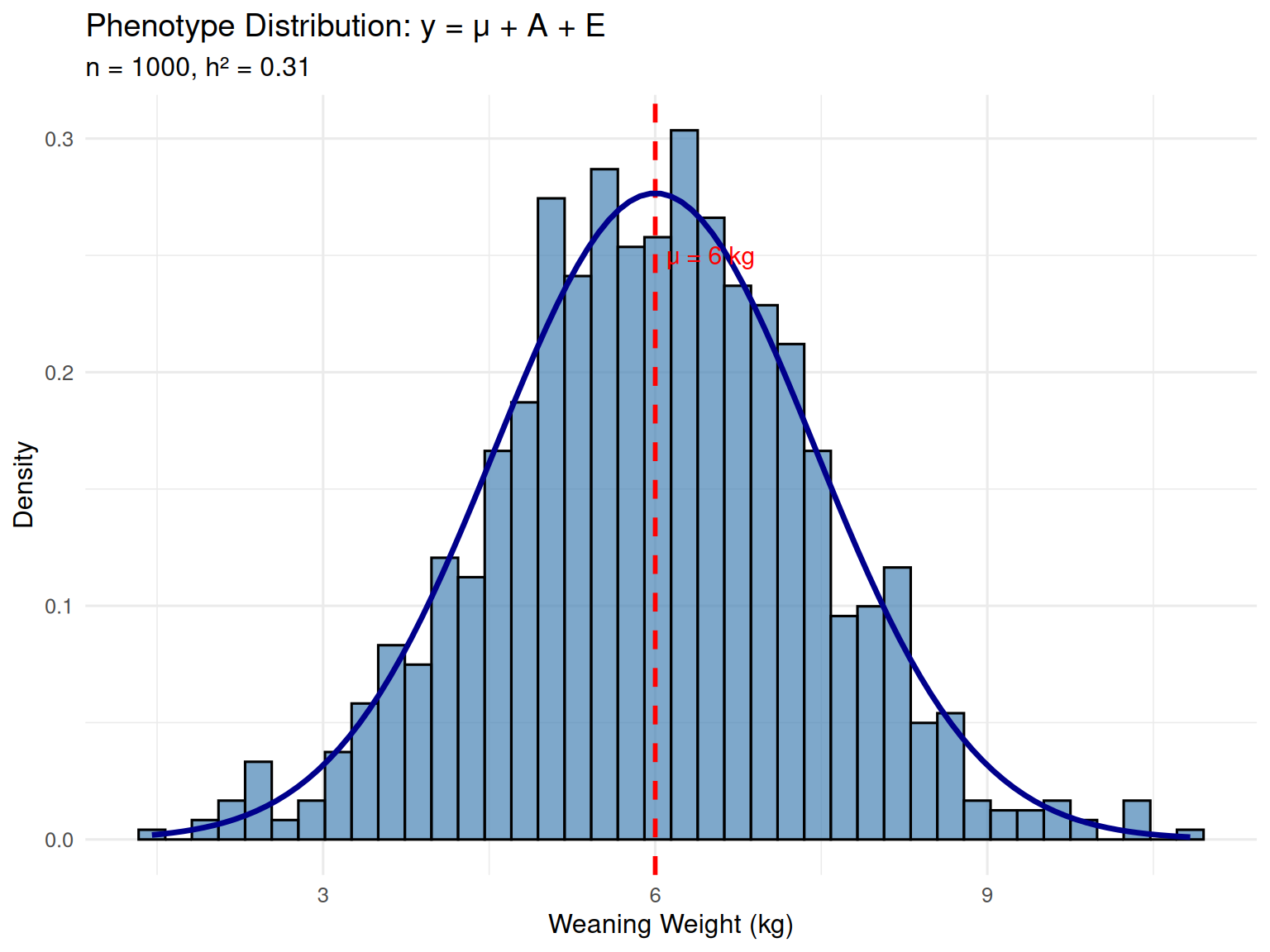
Interpretation:
- The histogram shows the distribution of phenotypes across the population
- The red dashed line marks the population mean (μ = 6.0 kg)
- The phenotypic distribution is approximately normal, as expected for a polygenic trait
- The phenotypic standard deviation (σ_P ≈ 1.44 kg) is larger than either the genetic (σ_A = 0.8 kg) or environmental (σ_E = 1.2 kg) SD alone—variation comes from both sources
3.8.2 Demonstration 2: Visualizing Variance Components
Let’s visualize how much of each animal’s phenotypic deviation from the mean is due to genetics vs. environment.
# Select 20 random animals for visualization
set.seed(123)
sample_animals <- population %>%
  slice_sample(n = 20) %>%
  arrange(phenotype) %>%
  mutate(animal_label = paste0("Animal ", row_number()))

# Create stacked bar plot showing A and E contributions
sample_animals_long <- sample_animals %>%
  select(animal_label, breeding_value, environment) %>%
  pivot_longer(cols = c(breeding_value, environment),
               names_to = "component",
               values_to = "value") %>%
  mutate(component = factor(component,
                            levels = c("breeding_value", "environment"),
                            labels = c("Genetic (A)", "Environmental (E)")))

ggplot(sample_animals_long, aes(x = animal_label, y = value, fill = component)) +
  geom_col(position = "stack") +
  geom_hline(yintercept = 0, linewidth = 0.5) +
  scale_fill_manual(values = c("Genetic (A)" = "#2E86AB",
                                "Environmental (E)" = "#A23B72")) +
  labs(title = "Genetic vs. Environmental Contributions to Phenotypic Deviation",
       subtitle = paste0("Deviation from population mean (μ = ", mu, " kg)"),
       x = "Animal",
       y = "Deviation from Mean (kg)",
       fill = "Component") +
  theme_minimal(base_size = 11) +
  theme(axis.text.x = element_text(angle = 45, hjust = 1),
        legend.position = "top")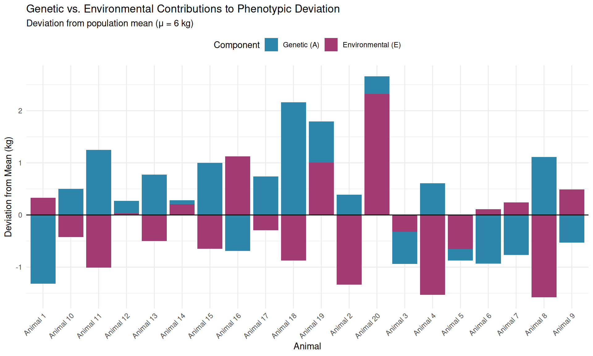
Interpretation:
- Each bar represents an animal’s total deviation from the population mean
- The blue portion (A) is the genetic contribution (breeding value)
- The pink portion (E) is the environmental contribution
- Some animals are above average due to good genetics (positive A) and/or favorable environment (positive E)
- Others are below average due to poor genetics (negative A) and/or unfavorable environment (negative E)
- The challenge in animal breeding is that we observe the total bar height (phenotype) but want to know the blue component (breeding value)
3.8.3 Demonstration 3: Comparing High vs. Low Heritability Traits
Let’s simulate two traits with different heritabilities to see how this affects the genetic vs. environmental contributions.
# High heritability trait (e.g., backfat depth in swine)
h2_high <- 0.60
sigma_P_high <- 3.0  # Phenotypic SD (mm)
sigma_A_high <- sqrt(h2_high * sigma_P_high^2)
sigma_E_high <- sqrt((1 - h2_high) * sigma_P_high^2)

# Low heritability trait (e.g., litter size in swine)
h2_low <- 0.12
sigma_P_low <- 2.5  # Phenotypic SD (piglets)
sigma_A_low <- sqrt(h2_low * sigma_P_low^2)
sigma_E_low <- sqrt((1 - h2_low) * sigma_P_low^2)

# Create data for visualization
variance_data <- data.frame(
  trait = rep(c("High h² (0.60)\nBackfat depth",
                "Low h² (0.12)\nLitter size"), each = 2),
  component = rep(c("Genetic (A)", "Environmental (E)"), 2),
  proportion = c(h2_high, 1 - h2_high, h2_low, 1 - h2_low),
  variance = c(sigma_A_high^2, sigma_E_high^2, sigma_A_low^2, sigma_E_low^2)
) %>%
  mutate(label = scales::percent(proportion, accuracy = 1))

# Create stacked bar chart comparison
ggplot(variance_data, aes(x = trait, y = proportion, fill = component)) +
  geom_col(width = 0.6) +
  geom_text(aes(label = label), position = position_stack(vjust = 0.5),
            color = "white", fontface = "bold", size = 5) +
  scale_fill_manual(values = c("Genetic (A)" = "#2E86AB",
                                "Environmental (E)" = "#A23B72")) +
  scale_y_continuous(labels = scales::percent, expand = c(0, 0)) +
  labs(title = "Variance Partitioning: High vs. Low Heritability Traits",
       subtitle = "Proportion of phenotypic variance due to genetics (A) vs. environment (E)",
       x = NULL,
       y = "Proportion of Phenotypic Variance",
       fill = "Component") +
  theme_minimal(base_size = 12) +
  theme(legend.position = "bottom",
        axis.text.x = element_text(size = 11, face = "bold"),
        panel.grid.major.x = element_blank())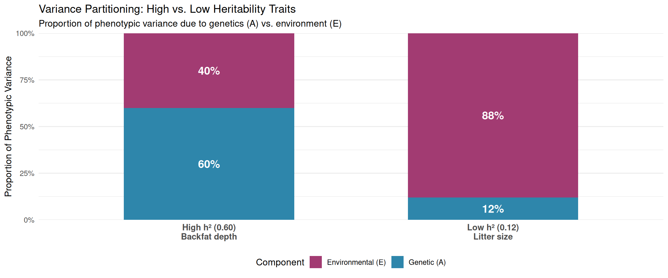
Interpretation:
High heritability trait (h² = 0.60, Backfat): - 60% of variation is genetic → phenotypes are good indicators of breeding values - 40% of variation is environmental - Selection is effective → choosing animals with low backfat usually means choosing animals with good genetics
Low heritability trait (h² = 0.12, Litter size): - Only 12% of variation is genetic → phenotypes are poor indicators of breeding values - 88% of variation is environmental → most differences between sows are due to luck - Selection is challenging → need many records and sophisticated methods (BLUP, genomic selection) to accurately estimate breeding values
3.8.4 Demonstration 4: Parent-Offspring Regression
Let’s simulate parent-offspring pairs and visualize the regression relationship, which provides an estimate of heritability.
# Function to simulate parent-offspring pairs
simulate_families <- function(n_families, h2, mu = 100, sigma_P = 15) {
  sigma_A <- sqrt(h2 * sigma_P^2)
  sigma_E <- sqrt((1 - h2) * sigma_P^2)

  # Simulate parents
  sires <- tibble(
    sire_id = 1:n_families,
    A_sire = rnorm(n_families, 0, sigma_A),
    E_sire = rnorm(n_families, 0, sigma_E),
    y_sire = mu + A_sire + E_sire
  )

  dams <- tibble(
    dam_id = 1:n_families,
    A_dam = rnorm(n_families, 0, sigma_A),
    E_dam = rnorm(n_families, 0, sigma_E),
    y_dam = mu + A_dam + E_dam
  )

  # Simulate offspring (5 per family)
  offspring_per_family <- 5
  offspring <- crossing(sire_id = 1:n_families, offspring_num = 1:offspring_per_family) %>%
    left_join(sires, by = "sire_id") %>%
    left_join(dams %>% rename(sire_id = dam_id), by = "sire_id") %>%
    mutate(
      # Offspring breeding value = midparent + Mendelian sampling
      A_midparent = (A_sire + A_dam) / 2,
      MS = rnorm(n(), 0, sqrt(0.5 * sigma_A^2)),
      A_offspring = A_midparent + MS,
      E_offspring = rnorm(n(), 0, sigma_E),
      y_offspring = mu + A_offspring + E_offspring,
      y_midparent = (y_sire + y_dam) / 2
    )

  return(offspring)
}

# Simulate for high and low heritability
set.seed(456)
n_families <- 100

high_h2_data <- simulate_families(n_families, h2 = 0.60) %>%
  mutate(trait = "High h² (0.60)")

low_h2_data <- simulate_families(n_families, h2 = 0.15) %>%
  mutate(trait = "Low h² (0.15)")

combined_data <- bind_rows(high_h2_data, low_h2_data)

# Fit regressions
regression_results <- combined_data %>%
  group_by(trait) %>%
  summarize(
    intercept = coef(lm(y_offspring ~ y_midparent))[1],
    slope = coef(lm(y_offspring ~ y_midparent))[2],
    r_squared = summary(lm(y_offspring ~ y_midparent))$r.squared,
    .groups = "drop"
  )

# Plot parent-offspring regressions
ggplot(combined_data, aes(x = y_midparent, y = y_offspring)) +
  geom_point(alpha = 0.4, size = 1.5, color = "steelblue") +
  geom_smooth(method = "lm", se = TRUE, color = "darkred", linewidth = 1.2) +
  geom_abline(intercept = 100, slope = 0, linetype = "dashed", color = "gray50") +
  facet_wrap(~ trait) +
  geom_text(data = regression_results,
            aes(x = 85, y = 125,
                label = paste0("Slope (h²) = ", round(slope, 2),
                              "\nR² = ", round(r_squared, 2))),
            hjust = 0, size = 4, color = "darkred", fontface = "bold") +
  labs(title = "Parent-Offspring Regression: Estimating Heritability",
       subtitle = "Regression slope equals heritability",
       x = "Midparent Phenotype",
       y = "Offspring Phenotype") +
  theme_minimal(base_size = 12) +
  theme(strip.text = element_text(size = 12, face = "bold"))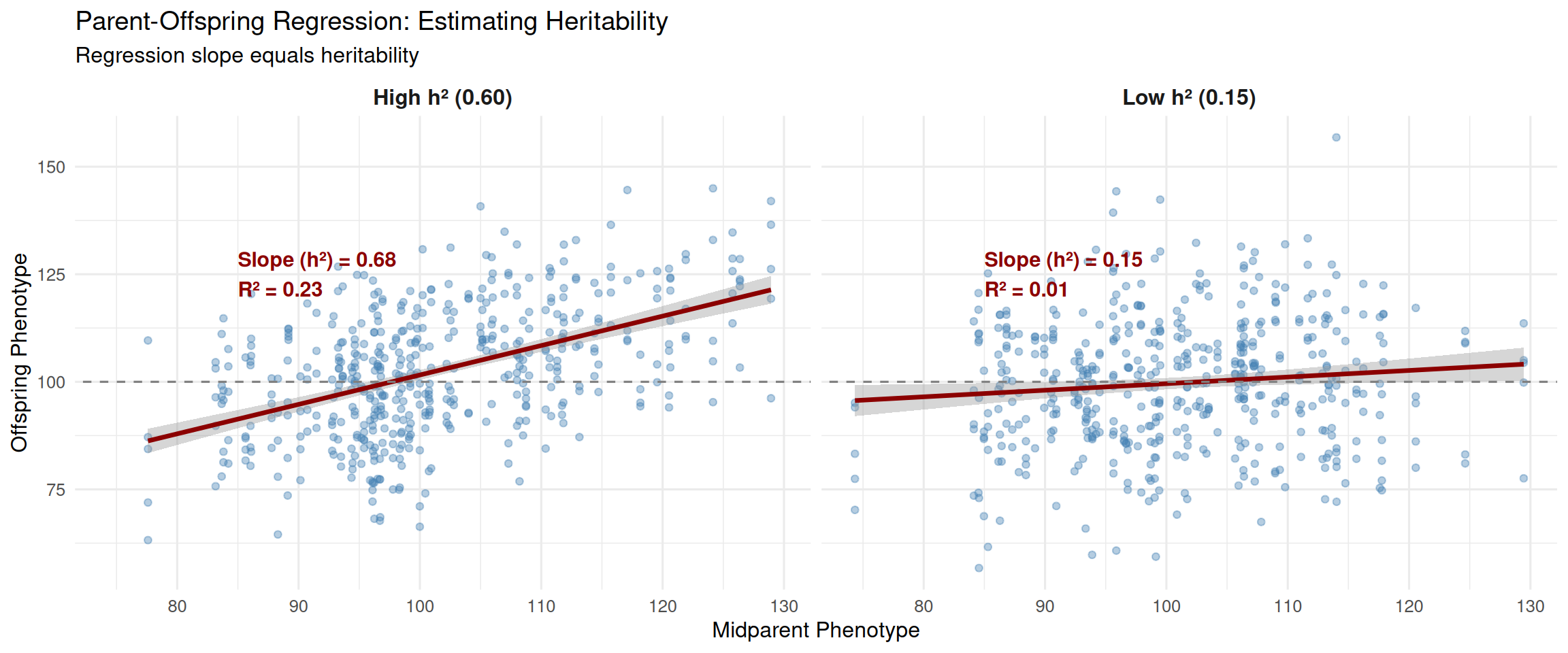
Interpretation:
High heritability (h² = 0.60): - Steep slope (β ≈ 0.60): Strong parent-offspring resemblance - High R² (≈ 0.35–0.40): Midparent phenotype explains substantial offspring variation - Points cluster tightly around the regression line - Implication: Selecting parents with high phenotypes is effective
Low heritability (h² = 0.15): - Shallow slope (β ≈ 0.15): Weak parent-offspring resemblance - Low R² (≈ 0.05–0.10): Midparent phenotype explains little offspring variation - Points are widely scattered around the regression line - Implication: Phenotypic selection is ineffective; need better breeding value estimates
The regression slope provides a classical estimate of heritability: \(\hat{h}^2 = \beta\).
3.8.5 Demonstration 5: The Power of BLUP vs. Phenotypic Selection
Let’s simulate a scenario comparing selection based on phenotype alone vs. selection based on estimated breeding values (simplified BLUP concept).
# Simulate population with moderate heritability
set.seed(789)
n_pop <- 200
h2_mod <- 0.35
mu_mod <- 100
sigma_P_mod <- 15
sigma_A_mod <- sqrt(h2_mod * sigma_P_mod^2)
sigma_E_mod <- sqrt((1 - h2_mod) * sigma_P_mod^2)

population_selection <- tibble(
  animal_id = 1:n_pop,
  A = rnorm(n_pop, 0, sigma_A_mod),
  E = rnorm(n_pop, 0, sigma_E_mod),
  y = mu_mod + A + E
) %>%
  mutate(
    # Simple EBV estimate: regression on phenotype
    EBV = h2_mod * (y - mu_mod),
    rank_phenotype = rank(-y),
    rank_EBV = rank(-EBV),
    rank_true_BV = rank(-A)
  )

# Select top 10% based on phenotype vs. EBV
prop_selected <- 0.10
n_selected <- round(n_pop * prop_selected)

selected_phenotype <- population_selection %>%
  slice_max(y, n = n_selected) %>%
  mutate(selection_method = "Phenotypic Selection")

selected_EBV <- population_selection %>%
  slice_max(EBV, n = n_selected) %>%
  mutate(selection_method = "EBV-Based Selection")

# Compare average true breeding value of selected animals
comparison <- bind_rows(
  selected_phenotype %>% summarize(mean_true_BV = mean(A), method = "Phenotype"),
  selected_EBV %>% summarize(mean_true_BV = mean(A), method = "EBV")
)

cat("Selection Comparison (Top 10% selected):\n\n")
Selection Comparison (Top 10% selected):cat("Phenotypic Selection:\n")Phenotypic Selection:cat(sprintf(" Mean true breeding value: %.2f\n",
comparison$mean_true_BV[comparison$method == "Phenotype"])) Mean true breeding value: 9.37cat("\nEBV-Based Selection:\n")
EBV-Based Selection:cat(sprintf(" Mean true breeding value: %.2f\n",
comparison$mean_true_BV[comparison$method == "EBV"])) Mean true breeding value: 9.37cat(sprintf("\nImprovement from using EBVs: %.2f%%\n",
100 * (comparison$mean_true_BV[comparison$method == "EBV"] -
comparison$mean_true_BV[comparison$method == "Phenotype"]) /
comparison$mean_true_BV[comparison$method == "Phenotype"]))
Improvement from using EBVs: 0.00%# Visualize
selected_combined <- bind_rows(selected_phenotype, selected_EBV)
ggplot(population_selection, aes(x = y, y = A)) +
geom_point(alpha = 0.3, size = 2, color = "gray60") +
geom_point(data = selected_combined,
aes(color = selection_method), size = 3, alpha = 0.8) +
geom_hline(yintercept = 0, linetype = "dashed", color = "black") +
geom_vline(xintercept = mu_mod, linetype = "dashed", color = "black") +
scale_color_manual(values = c("Phenotypic Selection" = "#E63946",
"EBV-Based Selection" = "#06A77D")) +
labs(title = "Phenotypic Selection vs. EBV-Based Selection",
subtitle = paste0("h² = ", h2_mod, ", selecting top ", prop_selected*100, "%"),
x = "Phenotype (y)",
y = "True Breeding Value (A)",
color = "Selection Method") +
annotate("text", x = 85, y = 12,
label = paste0("EBV selection captures\n",
round(100 * (comparison$mean_true_BV[2] - comparison$mean_true_BV[1]) /
comparison$mean_true_BV[1], 1),
"% more genetic merit"),
hjust = 0, color = "#06A77D", fontface = "bold") +
theme_minimal(base_size = 12) +
theme(legend.position = "top")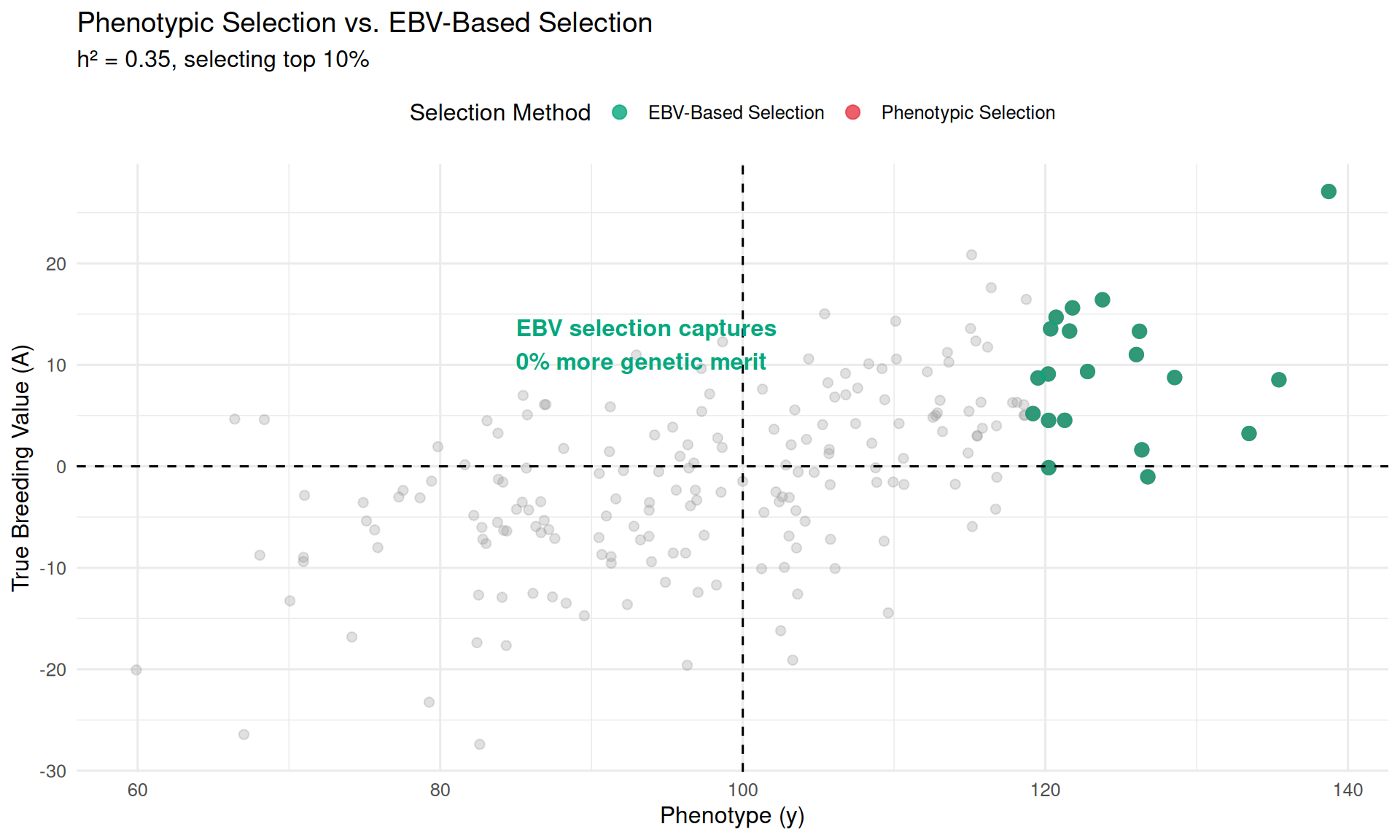
Interpretation:
- Gray points: All animals in the population
- Red points: Animals selected based on highest phenotypes
- Green points: Animals selected based on highest estimated breeding values (EBVs)
Key insights: 1. Phenotypic selection sometimes picks animals with high phenotypes due to favorable environments (high E), not high breeding values 2. EBV-based selection better identifies animals with truly superior genetics (high A), even if their phenotypes are moderate 3. The improvement from using EBVs instead of phenotypes is typically 5-20% more genetic progress, depending on heritability
This demonstrates why modern breeding programs invest in BLUP and genomic selection—they provide more accurate breeding value estimates, leading to faster genetic progress.
3.8.6 Key Takeaways from R Demonstrations
The basic model \(y = \mu + A + E\) can be simulated to create realistic phenotypic distributions
Variance components determine what proportion of phenotypic variation is genetic vs. environmental
Heritability affects selection efficiency: High h² → phenotype is reliable; Low h² → need sophisticated methods
Parent-offspring regression provides a classical method to estimate heritability from data
Breeding value estimation (BLUP, genomic selection) outperforms phenotypic selection by accounting for environmental effects
These simulations provide a foundation for understanding more advanced topics in later chapters, including BLUP (Chapter 7), selection response (Chapter 6), and genomic selection (Chapter 13).
3.9 Summary
This chapter introduced the fundamental genetic model that underlies all of quantitative genetics and animal breeding. Understanding how phenotypes are determined by the combination of genetic and environmental effects is essential for estimating breeding values, predicting response to selection, and designing effective breeding programs.
3.9.1 Key Points
The Basic Genetic Model
-
Phenotype is the sum of genetic and environmental effects: \(y = \mu + A + E\)
- \(y\) = observed phenotype (measurable)
- \(\mu\) = population mean (estimable)
- \(A\) = additive genetic effect or breeding value (must be estimated)
- \(E\) = environmental deviation (unmeasurable for individuals)
- The challenge of animal breeding is separating \(A\) from \(E\) so we can identify and select animals with superior genetic merit
Types of Genetic Effects
-
Genetic effects partition into three types: \(G = A + D + I\)
- Additive effects (\(A\)): Sum of average effects of alleles; breed true; determine breeding value
- Dominance effects (\(D\)): Within-locus interactions; don’t breed true; contribute to heterosis in crossbreeding
- Epistatic effects (\(I\)): Between-locus interactions; don’t breed true; largely unpredictable
-
Only additive effects matter for long-term genetic improvement because:
- They transmit predictably from parent to offspring: \(E(A_{offspring}) = \frac{1}{2}(A_{sire} + A_{dam})\)
- Response to selection depends on additive genetic variance (\(\sigma^2_A\)), not total genetic variance
- Dominance and epistasis “wash out” over generations—they don’t accumulate
Variance Partitioning
Phenotypic variance partitions into components: \(\sigma^2_P = \sigma^2_A + \sigma^2_D + \sigma^2_I + \sigma^2_E\)
In practice, we simplify to: \(\sigma^2_P = \sigma^2_A + \sigma^2_E\)
-
Heritability (\(h^2 = \sigma^2_A / \sigma^2_P\)) quantifies the proportion of phenotypic variance due to additive genetics
- High \(h^2\) (0.40–0.70): Production and carcass traits → effective selection
- Low \(h^2\) (0.05–0.20): Reproductive and fitness traits → challenging selection
Variance components are population-specific, not universal properties of traits
Parent-Offspring Relationships
Offspring inherit half of each parent’s breeding value on average, plus Mendelian sampling variation
Parent-offspring regression slope equals heritability: \(\beta = h^2\)
Regression toward the mean occurs because offspring don’t inherit environmental effects and inherit only half of parental genetic deviations
Practical Implications
Phenotypic selection is effective for high-h² traits but misleading for low-h² traits
Modern breeding methods (BLUP, genomic selection) estimate breeding values more accurately than phenotypic selection alone, especially for lowly heritable traits
Different species and traits require different breeding strategies based on heritability, generation interval, and reproductive rate
This chapter provides the theoretical foundation for the rest of the book. The concepts introduced here—breeding values, variance components, heritability—will be used throughout Chapters 5–13 as we develop more sophisticated selection and genomic methods.
3.10 Practice Problems
Work through these problems to test your understanding of the basic genetic model. Solutions are provided below.
3.10.1 Problems
A broiler chicken has a phenotype of 2,950 g for 42-day body weight. The population mean is 2,800 g, and the chicken’s breeding value is +80 g. What is the environmental deviation for this chicken?
Explain in your own words why dominance effects do not contribute to long-term response to selection, even though they affect individual phenotypes.
-
For a trait with \(\sigma^2_P = 100\) units², \(\sigma^2_A = 30\) units², and \(\sigma^2_E = 60\) units²:
- What is \(\sigma^2_D + \sigma^2_I\) (combined dominance and epistatic variance)?
- What is the heritability (\(h^2\)) if we use the simplified model \(\sigma^2_P = \sigma^2_A + \sigma^2_E\)?
A boar has a breeding value of +120 g/day for average daily gain. If he is mated to sows with an average breeding value of +60 g/day, what is the expected breeding value of their offspring?
In a dairy cattle population, the heritability of milk yield is 0.35. Two parents have phenotypes of 12,000 kg and 11,400 kg. The population mean is 10,500 kg. Using the simple regression method, estimate the expected breeding value of their offspring. (Hint: Midparent phenotype deviation × \(h^2\))
Why do full siblings (same sire and dam) have different phenotypes and different breeding values, even though they have the same expected breeding value?
-
A trait has phenotypic variance \(\sigma^2_P = 16\) kg² and heritability \(h^2 = 0.45\). Calculate:
- Additive genetic variance (\(\sigma^2_A\))
- Environmental variance (\(\sigma^2_E\))
- Additive genetic standard deviation (\(\sigma_A\))
Explain why heritability is a population parameter, not a trait parameter. Give an example of how the same trait could have different heritabilities in two populations.
3.10.2 Solutions
Problem 1
Using \(y = \mu + A + E\), we can solve for \(E\):
\[E = y - \mu - A = 2,950 - 2,800 - 80 = +70 \text{ g}\]
The chicken experienced a favorable environmental effect of +70 g (perhaps better feeder access or avoided early disease).
Problem 2
Dominance effects depend on specific genotype combinations at individual loci (having two different alleles creates the dominance effect). When parents reproduce, their alleles segregate and recombine with alleles from the other parent, creating new genotypes in offspring. The specific genotype combination that created the dominance effect in the parent is not preserved in the offspring—it’s “broken up” during meiosis and recombination.
Over generations of selection, we can increase the frequency of beneficial alleles (which changes additive genetic effects), but we cannot reliably select for favorable dominance combinations because they don’t transmit as stable entities. Therefore, dominance creates short-term variation in individual phenotypes but doesn’t contribute to long-term, cumulative genetic improvement.
Problem 3
- Using the full model: \(\sigma^2_P = \sigma^2_A + \sigma^2_D + \sigma^2_I + \sigma^2_E\)
\[\sigma^2_D + \sigma^2_I = \sigma^2_P - \sigma^2_A - \sigma^2_E = 100 - 30 - 60 = 10 \text{ units}^2\]
- Using the simplified model where we lump non-additive effects into environmental variance:
\[h^2 = \frac{\sigma^2_A}{\sigma^2_P} = \frac{30}{100} = 0.30\]
Note: The simplified model treats the 10 units² of dominance and epistatic variance as part of “environmental” (non-heritable) variation.
Problem 4
Offspring breeding value equals the midparent breeding value (on average):
\[E(A_{offspring}) = \frac{1}{2}A_{sire} + \frac{1}{2}A_{dam} = \frac{1}{2}(+120) + \frac{1}{2}(+60) = +90 \text{ g/day}\]
Individual offspring will deviate from +90 g/day due to Mendelian sampling, but across many offspring, the average will be +90 g/day.
Problem 5
Midparent phenotype: \[y_{midparent} = \frac{12,000 + 11,400}{2} = 11,700 \text{ kg}\]
Midparent deviation from population mean: \[y_{midparent} - \mu = 11,700 - 10,500 = +1,200 \text{ kg}\]
Estimated offspring breeding value (using simple regression): \[\hat{A}_{offspring} = h^2 \times (y_{midparent} - \mu) = 0.35 \times 1,200 = +420 \text{ kg}\]
Expected offspring phenotype: \[E(y_{offspring}) = \mu + \hat{A}_{offspring} = 10,500 + 420 = 10,920 \text{ kg}\]
(This assumes average environment for offspring. Individual offspring will vary due to Mendelian sampling and environmental effects.)
Problem 6
Full siblings have different phenotypes and breeding values for two reasons:
1. Mendelian sampling (different breeding values): Even though siblings have the same expected breeding value (midparent average), they sample different alleles from each parent during meiosis. At each locus, a sibling randomly receives one of the parent’s two alleles. With thousands of loci involved in quantitative traits, different siblings inherit different combinations, creating variation in breeding values. The variance among full-sib breeding values is \(\frac{1}{2}\sigma^2_A\).
2. Environmental effects (different phenotypes): Each sibling experiences unique environmental effects (\(E\)) that affect its phenotype. Even siblings raised in the same pen don’t have identical environments—they compete for feed, experience different health challenges, and undergo random developmental variation. These environmental differences create phenotypic variation even if siblings had identical breeding values.
Problem 7
\(\sigma^2_A = h^2 \times \sigma^2_P = 0.45 \times 16 = 7.2 \text{ kg}^2\)
\(\sigma^2_E = \sigma^2_P - \sigma^2_A = 16 - 7.2 = 8.8 \text{ kg}^2\)
\(\sigma_A = \sqrt{\sigma^2_A} = \sqrt{7.2} = 2.68 \text{ kg}\)
This means breeding values in the population have a standard deviation of 2.68 kg. About 68% of animals have breeding values within ±2.68 kg of the population mean.
Problem 8
Heritability is a population parameter because it depends on the amounts of genetic and environmental variation present in a specific population, not on the trait itself.
The same trait can have different heritabilities in different populations because:
Genetic variance (\(\sigma^2_A\)) can differ: - Populations with more genetic diversity (varied allele frequencies) have higher \(\sigma^2_A\) - Populations under long-term selection may have reduced \(\sigma^2_A\) as favorable alleles approach fixation - Small, inbred populations have lower \(\sigma^2_A\) than large, diverse populations
Environmental variance (\(\sigma^2_E\)) can differ: - Populations raised in uniform, controlled environments (e.g., commercial poultry) have low \(\sigma^2_E\) - Populations in variable environments (e.g., range beef cattle) have high \(\sigma^2_E\)
Example:
Consider weaning weight in swine:
Population A (Commercial nucleus herd): - Uniform management, controlled feeding, excellent health care - \(\sigma^2_A = 4.0\) kg² (maintained diversity) - \(\sigma^2_E = 3.0\) kg² (low environmental variation) - \(\sigma^2_P = 7.0\) kg² - \(h^2 = 4.0 / 7.0 = 0.57\)
Population B (Small, backyard herd): - Variable management, mixed feeding, inconsistent health care - \(\sigma^2_A = 2.0\) kg² (less genetic diversity due to small size) - \(\sigma^2_E = 8.0\) kg² (high environmental variation) - \(\sigma^2_P = 10.0\) kg² - \(h^2 = 2.0 / 10.0 = 0.20\)
The same trait (weaning weight) has dramatically different heritabilities (0.57 vs. 0.20) in the two populations due to differences in both genetic and environmental variance.
3.11 Further Reading
For deeper exploration of the concepts introduced in this chapter:
Classic textbooks:
-
Falconer, D. S., & Mackay, T. F. C. (1996). Introduction to Quantitative Genetics (4th ed.). Pearson.
- Chapter 7: Values and Means
- Chapter 8: Variance
- The foundational textbook in quantitative genetics; rigorous mathematical treatment
-
Lynch, M., & Walsh, B. (1998). Genetics and Analysis of Quantitative Traits. Sinauer Associates.
- Chapter 7: Resemblance Between Relatives
- Chapter 12: Short-term Changes in the Mean
- Comprehensive and mathematically detailed; excellent for advanced students
Applied animal breeding:
-
Bourdon, R. M. (2000). Understanding Animal Breeding (2nd ed.). Prentice Hall.
- Chapter 6: The Genetic Model for Quantitative Traits
- More accessible treatment with livestock examples
-
Mrode, R. A. (2014). Linear Models for the Prediction of Animal Breeding Values (3rd ed.). CABI.
- Chapter 1: Genetic Evaluation with Different Sources of Information
- Focuses on practical breeding value estimation
Recent reviews:
-
Hill, W. G. (2010). Understanding and using quantitative genetic variation. Philosophical Transactions of the Royal Society B, 365(1537), 73–85.
- Excellent overview of variance components and their interpretation
-
Walsh, B., & Lynch, M. (2018). Evolution and Selection of Quantitative Traits. Oxford University Press.
- Modern treatment of quantitative genetics with evolutionary perspective
Online resources:
-
Animal Breeding and Genomics eXtension articles: articles.extension.org/animal_breeding_genomics
- Practical articles on genetic evaluation in livestock
-
Beef Improvement Federation Guidelines: Available at beefimprovement.org
- Practical guidance on EPDs and genetic evaluation in beef cattle