# Install required packages
install.packages("MASS") # For generalized inverse: ginv()
install.packages("car") # For VIF, Type III SS
install.packages("emmeans") # For adjusted means
install.packages("multcomp") # For multiple contrasts
install.packages("lme4") # For mixed models (Week 14)1 Week 1: Course Overview & Computational Foundations
1.1 Why Build Our Own Solvers?
1.1.1 The Black Box Problem
Most students learn to analyze data by running commands like:
model <- lm(y ~ x)
summary(model)
While this approach gets results quickly, it creates several problems:
- Lack of understanding: What is
lm()actually doing? - Limited flexibility: Can’t modify methods for special situations
- Difficulty debugging: When results seem wrong, where do you look?
- Blind trust: How do you know the software is correct?
1.1.2 Our Philosophy: Understanding Through Building
In this course, we take a different approach:
- Learn the mathematics behind each method
- Derive estimators from first principles
- Build solvers manually using matrix operations
- Verify our results against established software
- Then use software with confidence and understanding
NoteWhy This Matters for Animal Breeding
In animal breeding, we work with:
- Large datasets (thousands to millions of animals)
- Complex relationships (pedigrees, genomic data)
- Special structures (repeated records, incomplete data)
- Custom models (not always available in standard software)
Understanding how methods work allows you to:
- Adapt methods for your specific problems
- Recognize when software makes incorrect assumptions
- Build custom solutions when needed
- Communicate effectively with statisticians and programmers
1.2 Linear Models in Animal Breeding
Before diving into the mathematics, let’s see where linear models appear in animal breeding and genetics.
1.2.1 Best Linear Unbiased Prediction (BLUP)
BLUP is the foundation of modern genetic evaluation. It estimates breeding values by solving a large system of linear equations called mixed model equations (MME).
For a simple sire model:
\[ \mathbf{y} = \mathbf{X}\boldsymbol{\beta} + \mathbf{Z}\mathbf{u} + \mathbf{e} \]
Where:
- \(\mathbf{y}\) = vector of observations (e.g., milk yields)
- \(\mathbf{X}\) = design matrix for fixed effects (e.g., herds, years)
- \(\boldsymbol{\beta}\) = vector of fixed effects
- \(\mathbf{Z}\) = incidence matrix relating observations to sires
- \(\mathbf{u}\) = vector of sire effects (breeding values)
- \(\mathbf{e}\) = vector of random errors
We’ll build toward this model throughout the course, starting with simpler fixed effects models.
1.2.2 Estimated Progeny Differences (EPDs)
EPDs in beef cattle are predictions of genetic merit based on performance data. They come from solving linear models that account for:
- Contemporary groups (fixed effects)
- Genetic relationships (random effects)
- Multiple traits (multivariate models)
1.2.3 Yield Deviations
In dairy cattle, yield deviations adjust cow records for:
- Herd-year-season effects
- Age at calving
- Days in milk
- Previous lactations
These adjustments use linear model equations.
1.2.4 Genomic Evaluations
Modern genomic selection uses linear models relating:
- Phenotypes (e.g., growth rate)
- Genotypes (SNP markers)
- Relationships (genomic relationship matrix)
ImportantAll These Methods Share a Common Foundation
Every method listed above relies on:
- Expressing the problem as a linear model
- Building appropriate design matrices
- Solving systems of linear equations
- Understanding properties of estimators (BLUE, BLUP)
This course teaches you those fundamental skills.
1.3 Setting Up Your Computing Environment
1.3.1 Installing R and RStudio
If you haven’t already:
- Download R from https://cran.r-project.org/
- Download RStudio from https://posit.co/download/rstudio-desktop/
- Install both in that order (R first, then RStudio)
1.3.2 Required R Packages
We’ll use several R packages throughout the course. Install them now:
Load the main package we’ll use in Week 1:
library(MASS) # For ginv() function1.3.3 Test Your Installation
Run this simple test:
# Create a simple matrix
A <- matrix(c(1, 2, 3, 4), nrow = 2, ncol = 2)
print(A)
[,1] [,2]
[1,] 1 3
[2,] 2 4# Compute its inverse
A_inv <- solve(A)
print(A_inv) [,1] [,2]
[1,] -2 1.5
[2,] 1 -0.5# Verify: A %*% A_inv should equal identity matrix
I <- A %*% A_inv
print(round(I, 10)) # Round to remove floating point errors [,1] [,2]
[1,] 1 0
[2,] 0 1If this runs without errors and produces the identity matrix, you’re ready to go!
1.4 Review of Matrix Operations
Let’s review the matrix operations we’ll use throughout this course.
1.4.1 Creating Matrices in R
# Create a vector
y <- c(25, 28, 26, 30, 27)
print(y)
[1] 25 28 26 30 27# Create a matrix by specifying elements
X <- matrix(c(1, 1, 1, 1, 1), nrow = 5, ncol = 1)
print(X) [,1]
[1,] 1
[2,] 1
[3,] 1
[4,] 1
[5,] 1# Create a matrix using cbind (column bind)
X2 <- matrix(c(1, 1, 1, 1, 1,
25, 28, 26, 30, 27), nrow = 5, ncol = 2)
print(X2) [,1] [,2]
[1,] 1 25
[2,] 1 28
[3,] 1 26
[4,] 1 30
[5,] 1 27# Check dimensions
dim(y) # Actually a vector, shown as NULLNULLdim(X) # 5 rows, 1 column[1] 5 1dim(X2) # 5 rows, 2 columns[1] 5 21.4.2 Matrix Transpose
The transpose of a matrix swaps rows and columns.
Notation: \(\mathbf{X}'\) or \(\mathbf{X}^\top\)
X <- matrix(c(1, 2, 3, 4, 5, 6), nrow = 2, ncol = 3)
print("Original matrix X (2x3):")
[1] "Original matrix X (2x3):"print(X) [,1] [,2] [,3]
[1,] 1 3 5
[2,] 2 4 6X_transpose <- t(X)
print("Transposed matrix X' (3x2):")[1] "Transposed matrix X' (3x2):"print(X_transpose) [,1] [,2]
[1,] 1 2
[2,] 3 4
[3,] 5 61.4.3 Matrix Multiplication
Matrix multiplication follows the rule: \((n \times k)\) matrix times \((k \times m)\) matrix equals \((n \times m)\) matrix.
The number of columns in the first matrix must equal the number of rows in the second matrix.
# Example 1: Vector times matrix
A <- matrix(c(1, 2, 3, 4), nrow = 2, ncol = 2)
v <- c(5, 6)

# v is 1x2 (row vector), A is 2x2
# Result should be 1x2
result1 <- v %*% A
print(result1)
[,1] [,2]
[1,] 17 39# Example 2: Matrix times vector
# A is 2x2, v as column vector is 2x1
# Result should be 2x1
result2 <- A %*% v
print(result2) [,1]
[1,] 23
[2,] 34# Example 3: Matrix times matrix
B <- matrix(c(1, 0, 0, 1), nrow = 2, ncol = 2)
result3 <- A %*% B
print(result3) [,1] [,2]
[1,] 1 3
[2,] 2 4
TipMatrix Multiplication in R
In R, use %*% for matrix multiplication, NOT *.
A * Bperforms element-wise multiplicationA %*% Bperforms matrix multiplication
1.4.4 Matrix Addition
Matrices of the same dimensions can be added element-wise.
A <- matrix(c(1, 2, 3, 4), nrow = 2, ncol = 2)
B <- matrix(c(5, 6, 7, 8), nrow = 2, ncol = 2)

C <- A + B
print(C)
[,1] [,2]
[1,] 6 10
[2,] 8 121.4.5 Identity Matrix
The identity matrix \(\mathbf{I}\) is a square matrix with 1’s on the diagonal and 0’s elsewhere.
Property: \(\mathbf{A}\mathbf{I} = \mathbf{I}\mathbf{A} = \mathbf{A}\)
# Create 3x3 identity matrix
I3 <- diag(3)
print(I3)
[,1] [,2] [,3]
[1,] 1 0 0
[2,] 0 1 0
[3,] 0 0 1# Verify property
A <- matrix(c(1, 2, 3, 4, 5, 6, 7, 8, 9), nrow = 3, ncol = 3)
print("A * I equals A:")[1] "A * I equals A:"print(A %*% I3) [,1] [,2] [,3]
[1,] 1 4 7
[2,] 2 5 8
[3,] 3 6 91.5 The Sample Mean as a Linear Model
Let’s start with the simplest possible linear model: estimating a sample mean.
1.5.1 The Statistical Model
Suppose we have \(n\) observations: \(y_1, y_2, \ldots, y_n\).
We can write this as:
\[ y_i = \mu + e_i, \quad i = 1, 2, \ldots, n \tag{1.1}\]
Where:
- \(y_i\) = observation \(i\) (scalar)
- \(\mu\) = population mean (scalar, unknown parameter to estimate)
- \(e_i\) = random error for observation \(i\) (scalar)
1.5.2 Assumptions
We assume:
- \(E(e_i) = 0\) (errors have mean zero)
- \(Var(e_i) = \sigma^2\) (constant variance)
- \(Cov(e_i, e_j) = 0\) for \(i \neq j\) (errors are independent)
1.5.3 Matrix Form
We can write this model in matrix form:
\[ \mathbf{y} = \mathbf{X}\boldsymbol{\beta} + \mathbf{e} \tag{1.2}\]
Where:
\(\mathbf{y}\) is an \(n \times 1\) vector of observations: \(\mathbf{y} = \begin{bmatrix} y_1 \\ y_2 \\ \vdots \\ y_n \end{bmatrix}\)
\(\mathbf{X}\) is an \(n \times 1\) design matrix of ones: \(\mathbf{X} = \begin{bmatrix} 1 \\ 1 \\ \vdots \\ 1 \end{bmatrix}\)
\(\boldsymbol{\beta}\) is a \(1 \times 1\) vector (scalar) containing \(\mu\): \(\boldsymbol{\beta} = [\mu]\)
\(\mathbf{e}\) is an \(n \times 1\) vector of errors: \(\mathbf{e} = \begin{bmatrix} e_1 \\ e_2 \\ \vdots \\ e_n \end{bmatrix}\)
1.5.4 Least Squares Estimator
The least squares estimator minimizes the sum of squared errors:
\[ SSE = \sum_{i=1}^{n} e_i^2 = \sum_{i=1}^{n} (y_i - \mu)^2 \]
Taking the derivative with respect to \(\mu\) and setting equal to zero:
\[ \frac{\partial SSE}{\partial \mu} = -2\sum_{i=1}^{n}(y_i - \mu) = 0 \]
Solving:
\[ \sum_{i=1}^{n}y_i = n\mu \]
\[ \hat{\mu} = \frac{1}{n}\sum_{i=1}^{n}y_i = \bar{y} \tag{1.3}\]
The least squares estimate of \(\mu\) is simply the sample mean!
1.5.5 Using the Normal Equations
The general form of the normal equations is:
\[ \mathbf{X}'\mathbf{X}\mathbf{b} = \mathbf{X}'\mathbf{y} \tag{1.4}\]
Where \(\mathbf{b}\) is our estimate of \(\boldsymbol{\beta}\).
For our mean model:
\[ \mathbf{X}'\mathbf{X} = \begin{bmatrix} 1 & 1 & \cdots & 1 \end{bmatrix} \begin{bmatrix} 1 \\ 1 \\ \vdots \\ 1 \end{bmatrix} = n \]
This is a \(1 \times 1\) matrix (scalar) equal to \(n\).
\[ \mathbf{X}'\mathbf{y} = \begin{bmatrix} 1 & 1 & \cdots & 1 \end{bmatrix} \begin{bmatrix} y_1 \\ y_2 \\ \vdots \\ y_n \end{bmatrix} = \sum_{i=1}^{n} y_i \]
The normal equation becomes:
\[ n \cdot b = \sum_{i=1}^{n} y_i \]
Solving:
\[ b = \frac{1}{n}\sum_{i=1}^{n} y_i = \bar{y} \]
Same result!
1.5.6 Solution Using Matrix Inverse
The general solution to the normal equations (when \(\mathbf{X}'\mathbf{X}\) is invertible) is:
\[ \mathbf{b} = (\mathbf{X}'\mathbf{X})^{-1}\mathbf{X}'\mathbf{y} \tag{1.5}\]
For our mean model:
\[ (\mathbf{X}'\mathbf{X})^{-1} = n^{-1} = \frac{1}{n} \]
Therefore:
\[ b = \frac{1}{n} \sum_{i=1}^{n} y_i = \bar{y} \]
NoteNOTATION ESTABLISHED
This is Week 1, where we establish notation used throughout all 15 weeks:
Vectors and Matrices:
- \(\mathbf{y}\) = response/observation vector (lowercase bold)
- \(\mathbf{X}\) = design matrix (uppercase bold)
- \(\boldsymbol{\beta}\) = parameter vector (Greek lowercase bold)
- \(\mathbf{b}\) = estimate vector (lowercase bold)
- \(\mathbf{e}\) = error/residual vector (lowercase bold)
- \(\mathbf{I}\) = identity matrix (uppercase bold)
Operators:
- \(\mathbf{A}'\) or \(\mathbf{A}^\top\) = transpose
- \(\mathbf{A}^{-1}\) = matrix inverse
- \(\mathbf{A}^{-}\) = generalized inverse (introduced Week 2)
Scalars:
- \(n\) = sample size
- \(p\) = number of parameters
- \(\sigma^2\) = variance
Statistical Quantities:
- \(SSE\) = sum of squares for error
- \(SST\) = total sum of squares
- \(SSM\) = model sum of squares
This notation will be maintained consistently. Any extensions will be clearly marked.
1.6 Small Numerical Example: Dairy Milk Yield
Let’s work through a complete example calculating the mean milk yield for 5 Holstein cows.
1.6.1 Data
Daily milk yield (kg/day) for 5 cows:
y <- c(25, 28, 26, 30, 27)
n <- length(y)

print(paste("Observations:", paste(y, collapse = ", ")))
[1] "Observations: 25, 28, 26, 30, 27"print(paste("Sample size n =", n))[1] "Sample size n = 5"1.6.2 Model
\[ y_i = \mu + e_i, \quad i = 1, 2, 3, 4, 5 \]
We want to estimate \(\mu\) (the mean milk yield).
1.6.3 Design Matrix
X <- matrix(1, nrow = n, ncol = 1)
print("Design matrix X:")
[1] "Design matrix X:"print(X) [,1]
[1,] 1
[2,] 1
[3,] 1
[4,] 1
[5,] 1print(paste("Dimensions:", nrow(X), "x", ncol(X)))[1] "Dimensions: 5 x 1"1.6.4 Compute X’X
XtX <- t(X) %*% X
print("X'X:")
[1] "X'X:"print(XtX) [,1]
[1,] 5As expected, \(\mathbf{X}'\mathbf{X} = n = 5\).
1.6.5 Compute X’y
Xty <- t(X) %*% y
print("X'y:")
[1] "X'y:"print(Xty) [,1]
[1,] 136This equals \(\sum y_i = 25 + 28 + 26 + 30 + 27 = 136\).
1.6.6 Solve Normal Equations
\[ \mathbf{X}'\mathbf{X} \mathbf{b} = \mathbf{X}'\mathbf{y} \] \[ 5b = 136 \] \[ b = \frac{136}{5} = 27.2 \]
# Method 1: Using matrix inverse
XtX_inv <- solve(XtX)  # Inverse of X'X
b <- XtX_inv %*% Xty
print("Estimate of mu:")
[1] "Estimate of mu:"print(b) [,1]
[1,] 27.2# Method 2: Direct calculation
b_direct <- sum(y) / n
print("Direct calculation (sample mean):")[1] "Direct calculation (sample mean):"print(b_direct)[1] 27.2Both methods give \(\hat{\mu} = 27.2\) kg/day.
1.6.7 Fitted Values and Residuals
# Fitted values: y_hat = X * b
y_hat <- X %*% b
print("Fitted values:")
[1] "Fitted values:"print(y_hat) [,1]
[1,] 27.2
[2,] 27.2
[3,] 27.2
[4,] 27.2
[5,] 27.2# Residuals: e = y - y_hat
residuals <- y - y_hat
print("Residuals:")[1] "Residuals:"print(residuals) [,1]
[1,] -2.2
[2,] 0.8
[3,] -1.2
[4,] 2.8
[5,] -0.2# Check: sum of residuals should be zero
print(paste("Sum of residuals:", sum(residuals)))[1] "Sum of residuals: -1.4210854715202e-14"Each fitted value is \(\hat{y}_i = \hat{\mu} = 27.2\).
The residuals are: \(e_i = y_i - 27.2\).
TipProperty of Least Squares
For any model with an intercept, the sum of residuals equals zero (within rounding error):
\[ \sum_{i=1}^{n} e_i = 0 \]
1.6.8 Sum of Squares
# Total sum of squares
y_bar <- mean(y)
SST <- sum((y - y_bar)^2)
print(paste("Total SS:", SST))
[1] "Total SS: 14.8"# Sum of squares for error
SSE <- sum(residuals^2)
print(paste("Error SS:", SSE))[1] "Error SS: 14.8"# Alternative calculation
SSE_alt <- t(residuals) %*% residuals
print(paste("Error SS (matrix form):", SSE_alt))[1] "Error SS (matrix form): 14.8"1.6.9 Verify Against lm()
Let’s verify our hand calculations match R’s lm() function:
# Fit using lm()
model <- lm(y ~ 1)  # Model with intercept only
summary(model)
Call:
lm(formula = y ~ 1)

Residuals:
   1    2    3    4    5
-2.2  0.8 -1.2  2.8 -0.2

Coefficients:
            Estimate Std. Error t value Pr(>|t|)
(Intercept)  27.2000     0.8602   31.62 5.96e-06 ***
---
Signif. codes:  0 '***' 0.001 '**' 0.01 '*' 0.05 '.' 0.1 ' ' 1

Residual standard error: 1.924 on 4 degrees of freedom
# Compare our estimate to lm()
print("Our estimate:")[1] "Our estimate:"print(b) [,1]
[1,] 27.2print("lm() estimate:")[1] "lm() estimate:"print(coef(model))(Intercept)
27.2 # Are they equal?
print(paste("Match:", all.equal(c(b), coef(model))))[1] "Match: names for current but not for target"Perfect match!
1.7 R Implementation: Building Our First Solver
Let’s create a reusable function to compute the mean using the linear model approach:
# Function to estimate mean using linear model framework
estimate_mean <- function(y) {

  # Sample size
  n <- length(y)

  # Design matrix (column of ones)
  X <- matrix(1, nrow = n, ncol = 1)

  # Compute X'X
  XtX <- t(X) %*% X

  # Compute X'y
  Xty <- t(X) %*% y

  # Solve normal equations: b = (X'X)^-1 X'y
  b <- solve(XtX) %*% Xty

  # Compute fitted values
  y_hat <- X %*% b

  # Compute residuals
  residuals <- y - y_hat

  # Compute SSE
  SSE <- sum(residuals^2)

  # Compute variance estimate
  # sigma^2 = SSE / (n - p) where p = 1
  sigma2_hat <- SSE / (n - 1)

  # Return results as list
  results <- list(
    estimate = c(b),
    fitted_values = c(y_hat),
    residuals = c(residuals),
    SSE = SSE,
    sigma2 = sigma2_hat,
    n = n
  )

  return(results)
}

# Test our function
test_data <- c(25, 28, 26, 30, 27)
results <- estimate_mean(test_data)

print("Results from our custom function:")
[1] "Results from our custom function:"print(results)$estimate
[1] 27.2
$fitted_values
[1] 27.2 27.2 27.2 27.2 27.2
$residuals
[1] -2.2 0.8 -1.2 2.8 -0.2
$SSE
[1] 14.8
$sigma2
[1] 3.7
$n
[1] 5This function computes everything using matrix operations, just as we’ll do for more complex models in later weeks.
1.8 Realistic Livestock Application
Let’s apply our method to a larger dairy dataset.
1.8.1 Scenario
A dairy researcher collects morning milk yield data from 30 Holstein cows to estimate the herd average production level. The data represents cows in similar stages of lactation (60-90 days in milk) under the same management system.
1.8.2 Generate Realistic Data
# Set seed for reproducibility
set.seed(123)

# Generate realistic milk yield data (kg/day)
# Mean around 27 kg, SD around 4 kg (typical for Holsteins)
n <- 30
true_mean <- 27
true_sd <- 4

milk_yield <- round(rnorm(n, mean = true_mean, sd = true_sd), 1)

# Ensure no negative values (biologically impossible)
milk_yield[milk_yield < 0] <- abs(milk_yield[milk_yield < 0])

print("Milk yield data (kg/day):")
[1] "Milk yield data (kg/day):"print(milk_yield) [1] 24.8 26.1 33.2 27.3 27.5 33.9 28.8 21.9 24.3 25.2 31.9 28.4 28.6 27.4 24.8
[16] 34.1 29.0 19.1 29.8 25.1 22.7 26.1 22.9 24.1 24.5 20.3 30.4 27.6 22.4 32.01.8.3 Exploratory Analysis
# Summary statistics
summary(milk_yield)
Min. 1st Qu. Median Mean 3rd Qu. Max.
19.10 24.35 26.70 26.81 28.95 34.10 # Standard deviation
sd(milk_yield)[1] 3.922696# Histogram
hist(milk_yield,
breaks = 10,
main = "Distribution of Milk Yield",
xlab = "Milk Yield (kg/day)",
ylab = "Frequency",
col = "lightblue",
border = "white")
abline(v = mean(milk_yield), col = "red", lwd = 2, lty = 2)
legend("topright", legend = "Sample Mean", col = "red", lty = 2, lwd = 2)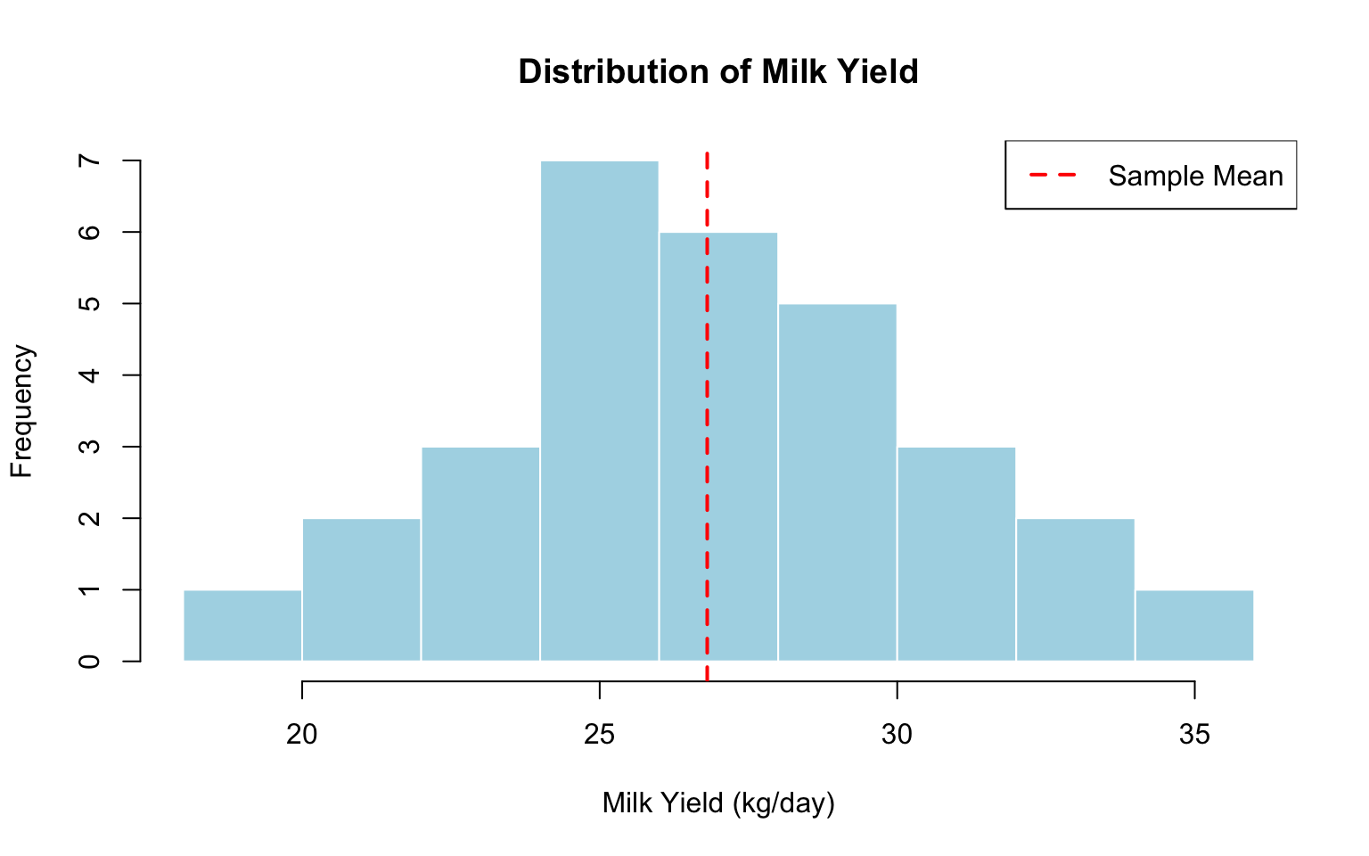
1.8.4 Estimate Mean Using Our Method
# Use our custom function
results_large <- estimate_mean(milk_yield)

print("Estimated mean milk yield:")
[1] "Estimated mean milk yield:"print(results_large$estimate)[1] 26.80667print("Estimated variance:")[1] "Estimated variance:"print(results_large$sigma2)[1] 15.38754print("Standard error of the mean:")[1] "Standard error of the mean:"se_mean <- sqrt(results_large$sigma2 / results_large$n)
print(se_mean)[1] 0.71618291.8.5 95% Confidence Interval
# Degrees of freedom
df <- n - 1

# Critical t-value (two-tailed, alpha = 0.05)
t_crit <- qt(0.975, df)

# Confidence interval
lower <- results_large$estimate - t_crit * se_mean
upper <- results_large$estimate + t_crit * se_mean

print(paste("95% CI: [", round(lower, 2), ",", round(upper, 2), "]"))
[1] "95% CI: [ 25.34 , 28.27 ]"1.8.6 Interpretation
The estimated mean milk yield is 26.81 kg/day with a 95% confidence interval of [25.34, 28.27] kg/day. This represents the average production level for this group of Holstein cows under these management conditions.
1.8.7 Compare with lm()
model_large <- lm(milk_yield ~ 1)
summary(model_large)
Call:
lm(formula = milk_yield ~ 1)

Residuals:
    Min      1Q  Median      3Q     Max
-7.7067 -2.4567 -0.1067  2.1433  7.2933

Coefficients:
            Estimate Std. Error t value Pr(>|t|)
(Intercept)  26.8067     0.7162   37.43   <2e-16 ***
---
Signif. codes:  0 '***' 0.001 '**' 0.01 '*' 0.05 '.' 0.1 ' ' 1

Residual standard error: 3.923 on 29 degrees of freedom
# Compare estimates
print("Our estimate vs lm():")[1] "Our estimate vs lm():"print(c(results_large$estimate, coef(model_large))) (Intercept)
26.80667 26.80667 # Check equality
all.equal(results_large$estimate, coef(model_large)[[1]])[1] TRUEPerfect agreement!
1.9 Connection to Breeding Applications
1.9.1 How This Relates to Genetic Evaluation
This simple example introduces concepts we’ll build on:
- Design matrices: We constructed \(\mathbf{X}\) from data structure
- Normal equations: We solved \(\mathbf{X}'\mathbf{X}\mathbf{b} = \mathbf{X}'\mathbf{y}\)
- Estimation: We obtained BLUE (Best Linear Unbiased Estimator)
- Variance: We estimated \(\sigma^2\) from residuals
In genetic evaluation:
- \(\mathbf{X}\) includes multiple fixed effects (herd, year, age, etc.)
- \(\mathbf{Z}\) relates observations to breeding values
- Normal equations become mixed model equations
- We estimate both fixed effects and predict breeding values
1.9.2 Preview: Contemporary Groups
In real breeding programs, we don’t estimate a single overall mean. Instead, we estimate means for contemporary groups - animals raised together under similar conditions.
For example:
- Herd-Year-Season groups in dairy
- Pen-Sex-Diet groups in swine
- Flock-Year-Management groups in sheep
Each group gets its own parameter in the design matrix. We’ll learn how to build these matrices in Week 3.
1.10 Summary
This week we:
- Established the course philosophy: understand through building
- Connected linear models to animal breeding applications
- Set up our computing environment
- Reviewed essential matrix operations
- Expressed the sample mean as a linear model
- Derived the least squares estimator using:
- Calculus (minimizing SSE)
- Normal equations (\(\mathbf{X}'\mathbf{X}\mathbf{b} = \mathbf{X}'\mathbf{y}\))
- Matrix inverse (\(\mathbf{b} = (\mathbf{X}'\mathbf{X})^{-1}\mathbf{X}'\mathbf{y}\))
- Implemented a solver function in R
- Verified results against
lm() - Applied the method to realistic dairy data
1.10.1 Key Takeaways
NoteWhat We Learned
- The sample mean is a special case of a linear model
- Matrix notation provides a unified framework
- Building solvers manually deepens understanding
- The methods scale from simple means to complex breeding value prediction
1.10.2 Looking Ahead
Next week (Week 2), we’ll dive deeper into linear algebra:
- Matrix rank and linear independence
- Regular and generalized inverses
- Solving systems of equations
- Properties critical for understanding estimability
This foundation will enable us to handle more complex models in subsequent weeks.
1.11 Additional Resources
1.11.1 R Documentation
?matrix- Creating matrices?solve- Matrix inverse?lm- Linear models
1.11.2 Recommended Reading
1.11.3 Practice Dataset
A CSV file with dairy milk yield data is available in the data/ subdirectory for additional practice.