---
title: "Week 3: Building the Design Matrix Framework"
format:
html:
toc: true
toc-depth: 3
number-sections: true
code-fold: false
code-tools: true
---
::: {.callout-note icon=false}
## Learning Objectives
By the end of this week, you will be able to:
1. **Construct** **design matrices** from raw data for different types of **predictors**
2. **Understand** and **apply** different **coding schemes** (**cell means model**, **effects model**, **reference cell coding**)
3. **Write** the **general linear model** in **matrix form** with correct notation
4. **State** and **interpret** the **assumptions** underlying linear models (**Gauss-Markov conditions**)
5. **Identify** when design matrices are **full rank** vs. **rank deficient**
6. **Build** design matrices manually in R and compare with `model.matrix()`
:::
## Introduction: From Raw Data to Matrix Representation
In Weeks 1 and 2, we established the computational foundations and reviewed the linear algebra essentials needed for linear models. Now we address the critical question: **How do we get from raw data to the matrix equations we solve?**
::: {.callout-important}
## The Bridge from Reality to Mathematics
The **design matrix** (denoted $\mathbf{X}$) is the bridge between:
- **Raw data**: Numbers in spreadsheets, databases, or field records
- **Mathematical model**: $\mathbf{y} = \mathbf{X}\boldsymbol{\beta} + \mathbf{e}$
Understanding how to construct $\mathbf{X}$ is fundamental to applying linear models in animal breeding and genetics.
:::
### Why This Matters in Animal Breeding
In animal breeding applications, we constantly work with different types of predictors:
- **Categorical factors**: Breed, sex, herd, diet, pen, treatment
- **Continuous covariates**: Birth weight, age, days in milk, temperature
- **Mixed models**: Contemporary groups (herd-year-season) combined with genetic relationships
The way we code these predictors into the design matrix determines:
1. **What parameters we estimate** (individual means vs. differences from baseline)
2. **Whether solutions are unique** (full rank vs. rank deficient)
3. **How we interpret results** (absolute effects vs. contrasts)
4. **Which hypotheses we can test** (estimable functions)
## The General Linear Model
### Matrix Form
The **general linear model** expresses the relationship between observations and parameters as:
$$
\mathbf{y} = \mathbf{X}\boldsymbol{\beta} + \mathbf{e}
$$
where:
- $\mathbf{y}$: $(n \times 1)$ vector of observations (response variable)
- $\mathbf{X}$: $(n \times p)$ design matrix (known constants)
- $\boldsymbol{\beta}$: $(p \times 1)$ vector of unknown parameters (to be estimated)
- $\mathbf{e}$: $(n \times 1)$ vector of random errors
::: {.callout-note}
## Dimensions Matter
Always verify matrix dimensions for compatibility:
- $\mathbf{X}$ is $n \times p$ (n observations, p parameters)
- $\boldsymbol{\beta}$ is $p \times 1$ (p parameters to estimate)
- $\mathbf{X}\boldsymbol{\beta}$ is $(n \times p)(p \times 1) = (n \times 1)$ ✓
- $\mathbf{y}$ is $n \times 1$ ✓
- $\mathbf{e}$ is $n \times 1$ ✓
The model equation is dimensionally consistent.
:::
### Expected Value Form
Taking expected values of both sides:
$$
E(\mathbf{y}) = E(\mathbf{X}\boldsymbol{\beta} + \mathbf{e}) = \mathbf{X}\boldsymbol{\beta} + E(\mathbf{e}) = \mathbf{X}\boldsymbol{\beta}
$$
This assumes $E(\mathbf{e}) = \mathbf{0}$ (errors have mean zero, discussed below).
### Scalar Form for Individual Observations
For the $i$-th observation:
$$
y_i = \sum_{j=1}^{p} x_{ij}\beta_j + e_i = x_{i1}\beta_1 + x_{i2}\beta_2 + \cdots + x_{ip}\beta_p + e_i
$$
where $x_{ij}$ is the element in row $i$, column $j$ of $\mathbf{X}$.
## Building Design Matrices for Different Predictor Types
The structure of $\mathbf{X}$ depends on the type of predictors in your model. Let's examine the three main types.
### Continuous Predictors (Regression)
When all predictors are continuous variables, the design matrix includes:
1. A column of ones (for the intercept)
2. Columns for each predictor variable
#### Example: Simple Linear Regression
Model: $y_i = \beta_0 + \beta_1 x_i + e_i$
For $n=4$ observations:
```{r}
#| label: continuous-example
#| message: false
# Data: broiler weight (kg) vs. age (days)
age <- c(21, 28, 35, 42)
weight <- c(0.5, 0.9, 1.4, 1.9)

# Design matrix: first column is intercept, second is predictor
X <- cbind(1, age)
print(X)
# Check dimensions
cat("\nDimensions: n =", nrow(X), "observations, p =", ncol(X), "parameters\n")
```
The design matrix is:
$$
\mathbf{X} = \begin{bmatrix}
1 & 21 \\
1 & 28 \\
1 & 35 \\
1 & 42
\end{bmatrix}_{4 \times 2}
$$
The parameter vector is:
$$
\boldsymbol{\beta} = \begin{bmatrix}
\beta_0 \\
\beta_1
\end{bmatrix}_{2 \times 1}
$$
#### Multiple Regression
With multiple continuous predictors: $y_i = \beta_0 + \beta_1 x_{1i} + \beta_2 x_{2i} + \cdots + \beta_k x_{ki} + e_i$
```{r}
#| label: multiple-continuous
# Example: Predict lamb weaning weight from birth weight and dam age
birth_wt <- c(4.5, 4.0, 4.8, 4.2, 4.6)
dam_age <- c(3, 5, 4, 6, 4)
wean_wt <- c(28, 24, 30, 26, 29)

# Design matrix: intercept, birth weight, dam age
X_mult <- cbind(1, birth_wt, dam_age)
colnames(X_mult) <- c("Intercept", "BirthWt", "DamAge")
print(X_mult)
```
$$
\mathbf{X} = \begin{bmatrix}
1 & 4.5 & 3 \\
1 & 4.0 & 5 \\
1 & 4.8 & 4 \\
1 & 4.2 & 6 \\
1 & 4.6 & 4
\end{bmatrix}_{5 \times 3}, \quad
\boldsymbol{\beta} = \begin{bmatrix}
\beta_0 \\
\beta_1 \\
\beta_2
\end{bmatrix}_{3 \times 1}
$$
### Categorical Predictors (ANOVA)
Categorical predictors (factors) require **indicator variables** (also called dummy variables). There are two primary coding schemes.
#### Cell Means Model
The **cell means model** estimates a separate mean for each group, with no explicit intercept.
Model: $y_{ij} = \mu_i + e_{ij}$
where $\mu_i$ is the mean for group $i$ ($i = 1, \ldots, g$ groups).
The design matrix has **one column per group**, with indicators for group membership:
$$
x_{ij} = \begin{cases}
1 & \text{if observation } j \text{ is in group } i \\
0 & \text{otherwise}
\end{cases}
$$
#### Example: Pig Litter Size by Breed (Cell Means)
```{r}
#| label: cell-means-example
#| message: false
# Load the pig data
pig_data <- data.frame(
  breed = c("Yorkshire", "Yorkshire", "Landrace", "Landrace", "Duroc", "Duroc"),
  litter_size = c(11, 12, 10, 11, 9, 10)
)

print(pig_data)
# Cell means design matrix: one column per breed
# Yorkshire = column 1, Landrace = column 2, Duroc = column 3
X_cell <- model.matrix(~ breed - 1, data = pig_data)  # -1 removes intercept
print(X_cell)
# Check rank
cat("\nRank of X:", qr(X_cell)$rank, "\n")
cat("Number of parameters:", ncol(X_cell), "\n")
```
The cell means design matrix is:
$$
\mathbf{X}_{\text{cell}} = \begin{bmatrix}
1 & 0 & 0 \\
1 & 0 & 0 \\
0 & 1 & 0 \\
0 & 1 & 0 \\
0 & 0 & 1 \\
0 & 0 & 1
\end{bmatrix}_{6 \times 3}
$$
Parameter vector:
$$
\boldsymbol{\beta}_{\text{cell}} = \begin{bmatrix}
\mu_{\text{Duroc}} \\
\mu_{\text{Landrace}} \\
\mu_{\text{Yorkshire}}
\end{bmatrix}_{3 \times 1}
$$
::: {.callout-tip}
## Cell Means Model Properties
- **Always full rank**: $r(\mathbf{X}) = p$ (number of groups)
- **Direct interpretation**: $\mu_i$ is the mean for group $i$
- **All parameters estimable**: Each $\mu_i$ can be uniquely estimated
- **Common in animal breeding**: Natural for comparing breed means, treatment means, etc.
:::
#### Effects Model (with Constraints)
The **effects model** decomposes each observation into an overall mean plus group-specific deviations.
Model: $y_{ij} = \mu + \alpha_i + e_{ij}$
where:
- $\mu$: overall mean (intercept)
- $\alpha_i$: effect of group $i$ (deviation from overall mean)
**Problem**: This model is **overparameterized** without constraints.
With $g$ groups, we have $g+1$ parameters ($\mu$ and $\alpha_1, \ldots, \alpha_g$), but only $g$ distinct means. We need a **constraint** to make parameters identifiable.
**Common constraint**: $\sum_{i=1}^{g} \alpha_i = 0$ (sum-to-zero constraint)
With this constraint, $\alpha_i$ represents the deviation of group $i$ from the overall mean.
#### Example: Pig Litter Size by Breed (Effects Model)
```{r}
#| label: effects-model-example
# Effects model design matrix: intercept + group indicators
# R uses reference cell coding by default (first level = 0)
X_effects <- model.matrix(~ breed, data = pig_data)
print(X_effects)
# Check rank
cat("\nRank of X:", qr(X_effects)$rank, "\n")
cat("Number of parameters:", ncol(X_effects), "\n")
```
The effects model design matrix (without constraint applied yet):
$$
\mathbf{X}_{\text{effects}} = \begin{bmatrix}
1 & 0 & 0 \\
1 & 0 & 0 \\
1 & 1 & 0 \\
1 & 1 & 0 \\
1 & 0 & 1 \\
1 & 0 & 1
\end{bmatrix}_{6 \times 3}
$$
::: {.callout-warning}
## Rank Deficiency Alert
The full effects model matrix (with all $g+1$ parameters) would be:
$$
\mathbf{X}_{\text{full}} = \begin{bmatrix}
1 & 1 & 0 & 0 \\
1 & 1 & 0 & 0 \\
1 & 0 & 1 & 0 \\
1 & 0 & 1 & 0 \\
1 & 0 & 0 & 1 \\
1 & 0 & 0 & 1
\end{bmatrix}_{6 \times 4}
$$
This has rank $r(\mathbf{X}) = 3 < 4$, making it **rank deficient**. Individual parameters ($\mu$, $\alpha_i$) are not uniquely estimable, but **contrasts** like $\alpha_i - \alpha_j$ are estimable.
We'll address non-full rank models in detail in Week 12.
:::
#### Reference Cell Coding (Set-to-Zero Constraint)
R's default for categorical variables uses **reference cell coding** (also called treatment coding):
- Set the first group's effect to zero: $\alpha_1 = 0$
- Other $\alpha_i$ represent deviations from group 1
With this constraint:
- $\mu$ = mean of reference group (Duroc, alphabetically first)
- $\alpha_{\text{Landrace}}$ = Landrace effect = (Landrace mean) - (Duroc mean)
- $\alpha_{\text{Yorkshire}}$ = Yorkshire effect = (Yorkshire mean) - (Duroc mean)
```{r}
#| label: reference-cell-interpretation
# Compute group means
group_means <- tapply(pig_data$litter_size, pig_data$breed, mean)
print(group_means)
# Interpretation with Duroc as reference (first alphabetically)
cat("\nWith reference cell coding (Duroc as baseline):\n")
cat("μ (intercept) = Duroc mean =", group_means["Duroc"], "\n")
cat("α_Landrace = Landrace - Duroc =", group_means["Landrace"] - group_means["Duroc"], "\n")
cat("α_Yorkshire = Yorkshire - Duroc =", group_means["Yorkshire"] - group_means["Duroc"], "\n")
```
### Mixed Predictors (ANCOVA)
When models include both categorical and continuous predictors, we have **Analysis of Covariance (ANCOVA)**.
Model: $y_{ij} = \mu + \alpha_i + \beta(x_{ij} - \bar{x}) + e_{ij}$
The design matrix combines indicator columns (for groups) and continuous columns (for covariates).
#### Example: Egg Production by Strain, Adjusted for Body Weight
```{r}
#| label: ancova-example
# Data: egg production (eggs/month) by strain, with body weight covariate
egg_data <- data.frame(
  strain = rep(c("Strain1", "Strain2", "Strain3"), each = 3),
  body_weight = c(1.8, 2.0, 1.9, 1.7, 1.8, 1.9, 2.1, 2.3, 2.2),
  eggs = c(24, 26, 25, 22, 23, 24, 26, 28, 27)
)

# ANCOVA design matrix: strain indicators + centered body weight
egg_data$bw_centered <- egg_data$body_weight - mean(egg_data$body_weight)
X_ancova <- model.matrix(~ strain + bw_centered, data = egg_data)
print(X_ancova)
```
::: {.callout-note}
## Centering Covariates
We often **center** continuous covariates by subtracting the mean: $x_{ij}^* = x_{ij} - \bar{x}$
**Benefits**:
1. The intercept represents the group mean at the average covariate value
2. Reduces collinearity between interaction terms and main effects
3. Makes parameter interpretation more intuitive
**Note**: Centering does NOT change $R^2$, residuals, or fitted values—only the interpretation of $\beta_0$.
:::
## Model Assumptions (Gauss-Markov Conditions)
For the general linear model $\mathbf{y} = \mathbf{X}\boldsymbol{\beta} + \mathbf{e}$, we make specific assumptions about the error term $\mathbf{e}$.
### The Three Core Assumptions
::: {.callout-important}
## Gauss-Markov Assumptions
Under these assumptions, ordinary least squares (OLS) estimators are BLUE (Best Linear Unbiased Estimators):
1. **Linearity**: The relationship between $\mathbf{y}$ and $\mathbf{X}$ is linear
- Correctly specified: $E(\mathbf{y}) = \mathbf{X}\boldsymbol{\beta}$
2. **Zero Mean Errors**: $E(\mathbf{e}) = \mathbf{0}$
- Errors are unbiased (centered at zero)
- No systematic over- or under-prediction
3. **Homoscedasticity and Independence**: $\text{Var}(\mathbf{e}) = \sigma^2\mathbf{I}$
- **Homoscedasticity**: Constant variance across all observations ($\text{Var}(e_i) = \sigma^2$ for all $i$)
- **Independence**: Errors are uncorrelated ($\text{Cov}(e_i, e_j) = 0$ for $i \neq j$)
:::
### Variance-Covariance Structure
The assumption $\text{Var}(\mathbf{e}) = \sigma^2\mathbf{I}$ can be written explicitly:
$$
\text{Var}(\mathbf{e}) = \begin{bmatrix}
\sigma^2 & 0 & 0 & \cdots & 0 \\
0 & \sigma^2 & 0 & \cdots & 0 \\
0 & 0 & \sigma^2 & \cdots & 0 \\
\vdots & \vdots & \vdots & \ddots & \vdots \\
0 & 0 & 0 & \cdots & \sigma^2
\end{bmatrix} = \sigma^2 \mathbf{I}
$$
- **Diagonal elements**: $\text{Var}(e_i) = \sigma^2$ (constant variance)
- **Off-diagonal elements**: $\text{Cov}(e_i, e_j) = 0$ (independence)
### Additional Assumption for Inference: Normality
For hypothesis testing and confidence intervals, we often add:
4. **Normality**: $\mathbf{e} \sim N(\mathbf{0}, \sigma^2\mathbf{I})$
This implies $\mathbf{y} \sim N(\mathbf{X}\boldsymbol{\beta}, \sigma^2\mathbf{I})$
::: {.callout-note}
## When is Normality Needed?
- **NOT needed** for unbiasedness of $\hat{\boldsymbol{\beta}}$ or minimum variance (Gauss-Markov)
- **IS needed** for:
- Exact $t$-tests and $F$-tests
- Confidence intervals with stated coverage
- Maximum likelihood interpretation
For large samples, the Central Limit Theorem provides approximate normality even if errors aren't exactly normal.
:::
### Violations and Consequences
| Violation | Consequence | Solution |
|-----------|-------------|----------|
| Non-linearity | Biased estimates | Transform variables, add polynomial terms |
| $E(\mathbf{e}) \neq \mathbf{0}$ | Biased intercept | Check model specification |
| Heteroscedasticity | Inefficient estimates, incorrect SEs | Weighted least squares, robust SEs |
| Correlation (e.g., time series) | Inefficient estimates, incorrect SEs | Generalized least squares, mixed models |
| Non-normality | Invalid inference (test statistics) | Transformations, bootstrapping, larger samples |
We'll explore diagnostics to check these assumptions in Week 11.
## Small Example: Pig Litter Size by Breed
Let's work through a complete small example, showing both cell means and effects model formulations.
### Data
```{r}
#| label: small-example-data
# Read the data
pig_data <- read.csv("data/pig_litter_breeds.csv")
print(pig_data)
# Summary statistics by breed
cat("\nSummary by breed:\n")
by(pig_data$litter_size, pig_data$breed, function(x) {
  cat(sprintf("  n = %d, mean = %.2f, sd = %.2f\n", length(x), mean(x), sd(x)))
})
```
### Cell Means Model
Model: $y_{ij} = \mu_i + e_{ij}$ where $i \in \{\text{Duroc, Landrace, Yorkshire}\}$
```{r}
#| label: small-example-cell-means
# Construct design matrix manually
n <- nrow(pig_data)
X_cell <- matrix(0, nrow = n, ncol = 3)
X_cell[pig_data$breed == "Duroc", 1] <- 1
X_cell[pig_data$breed == "Landrace", 2] <- 1
X_cell[pig_data$breed == "Yorkshire", 3] <- 1
colnames(X_cell) <- c("Duroc", "Landrace", "Yorkshire")

cat("Cell Means Design Matrix:\n")
print(X_cell)
# Response vector
y <- pig_data$litter_size

# Normal equations: X'X b = X'y
XtX <- t(X_cell) %*% X_cell
Xty <- t(X_cell) %*% y

cat("\nX'X (3×3):\n")
print(XtX)
cat("\nX'y (3×1):\n")
print(Xty)
# Solve for estimates
b_cell <- solve(XtX) %*% Xty
cat("\nParameter estimates:\n")
print(b_cell)
# These are just the group means!
cat("\nVerify these equal group means:\n")
print(tapply(y, pig_data$breed, mean))
```
**Interpretation**:
- $\hat{\mu}_{\text{Duroc}} = 9.5$ piglets per litter
- $\hat{\mu}_{\text{Landrace}} = 10.5$ piglets per litter
- $\hat{\mu}_{\text{Yorkshire}} = 11.5$ piglets per litter
::: {.callout-tip}
## Cell Means = Group Means
In the cell means model with balanced data, the estimates are simply the group means. The math gives us:
$$
\hat{\mu}_i = \frac{\sum_{j=1}^{n_i} y_{ij}}{n_i} = \bar{y}_{i\cdot}
$$
This is intuitive: our best estimate of a group's mean is the average of observations in that group!
:::
### Effects Model (Reference Cell Coding)
Model: $y_{ij} = \mu + \alpha_i + e_{ij}$ with $\alpha_{\text{Duroc}} = 0$ (Duroc as reference)
```{r}
#| label: small-example-effects
# Use R's default reference cell coding
X_effects <- model.matrix(~ breed, data = pig_data)

cat("Effects Model Design Matrix:\n")
print(X_effects)
# Note: Duroc is reference (alphabetically first), so no column for it
# breedLandrace and breedYorkshire are deviations from Duroc

# Solve using lm() for comparison
fit_effects <- lm(litter_size ~ breed, data = pig_data)
cat("\nParameter estimates (reference cell coding):\n")
print(coef(fit_effects))
# Manual calculation
XtX_eff <- t(X_effects) %*% X_effects
Xty_eff <- t(X_effects) %*% y
b_effects <- solve(XtX_eff) %*% Xty_eff

cat("\nManual calculation:\n")
print(b_effects)
```
**Interpretation (with Duroc as reference)**:
- $\hat{\mu} = 9.5$ = Duroc mean (reference group)
- $\hat{\alpha}_{\text{Landrace}} = 1.0$ = Landrace mean - Duroc mean = $10.5 - 9.5$
- $\hat{\alpha}_{\text{Yorkshire}} = 2.0$ = Yorkshire mean - Duroc mean = $11.5 - 9.5$
### Comparing the Two Models
```{r}
#| label: compare-models
# Cell means model: estimates are group means
cat("Cell Means Model Estimates:\n")
cat("Duroc:", b_cell[1], "\n")
cat("Landrace:", b_cell[2], "\n")
cat("Yorkshire:", b_cell[3], "\n\n")
# Effects model: reconstruct group means
cat("Effects Model - Reconstructed Group Means:\n")
cat("Duroc (reference):", b_effects[1], "\n")
cat("Landrace:", b_effects[1] + b_effects[2], "\n")
cat("Yorkshire:", b_effects[1] + b_effects[3], "\n\n")
# Both give identical fitted values
fitted_cell <- X_cell %*% b_cell
fitted_effects <- X_effects %*% b_effects

cat("Fitted values match:", all.equal(fitted_cell[,1], fitted_effects[,1]), "\n")
```
::: {.callout-important}
## Key Insight: Coding Doesn't Change Predictions
Different coding schemes (cell means vs. effects model) give different parameter estimates, but:
1. **Fitted values** $\hat{\mathbf{y}} = \mathbf{X}\hat{\boldsymbol{\beta}}$ are identical
2. **Residuals** $\mathbf{e} = \mathbf{y} - \hat{\mathbf{y}}$ are identical
3. **$R^2$**, **SSE**, and all other model fit statistics are identical
4. **Estimable functions** (like breed differences) give the same results
The choice of coding affects **parameter interpretation**, not model fit.
:::
## Realistic Application: Broiler Body Weight by Sex
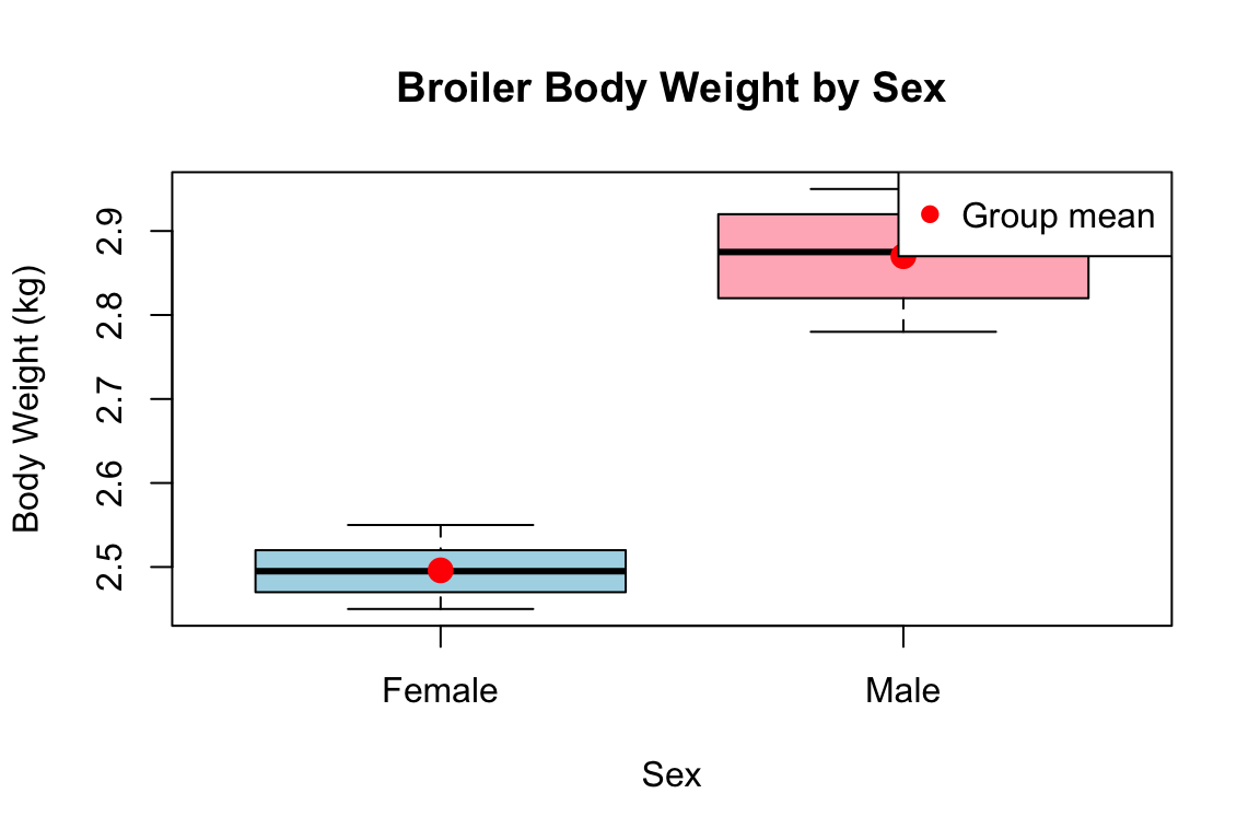
Now let's analyze a larger dataset: body weight (kg) for 20 broiler chickens at 42 days of age, by sex.
### Exploratory Analysis
```{r}
#| label: broiler-data
#| message: false
# Load data
broiler_data <- read.csv("data/broiler_bodyweight_sex.csv")

cat("Data structure:\n")
str(broiler_data)
cat("\nFirst few rows:\n")
head(broiler_data)
# Summary statistics by sex
cat("\nSummary statistics by sex:\n")
by(broiler_data$body_weight_kg, broiler_data$sex, function(x) {
  cat(sprintf("  n = %d, mean = %.3f, sd = %.3f, min = %.3f, max = %.3f\n",
              length(x), mean(x), sd(x), min(x), max(x)))
})
```
### Visualization
```{r}
#| label: broiler-plot
#| fig-width: 6
#| fig-height: 4
# Box plot
boxplot(body_weight_kg ~ sex, data = broiler_data,
        main = "Broiler Body Weight by Sex",
        xlab = "Sex",
        ylab = "Body Weight (kg)",
        col = c("lightblue", "lightpink"))

# Add means
means <- tapply(broiler_data$body_weight_kg, broiler_data$sex, mean)
points(1:2, means, pch = 19, col = "red", cex = 1.5)
legend("topright", legend = "Group mean", pch = 19, col = "red")
```
**Observations**:
- Males are clearly heavier than females (sexual dimorphism)
- Both groups show similar variation (standard deviations)
- Distributions appear roughly symmetric (no obvious outliers)
### Cell Means Model Analysis
```{r}
#| label: broiler-cell-means
# Cell means model: estimate mean for each sex
X_cell_broiler <- model.matrix(~ sex - 1, data = broiler_data)
y_broiler <- broiler_data$body_weight_kg

# Solve normal equations
XtX_broiler <- t(X_cell_broiler) %*% X_cell_broiler
Xty_broiler <- t(X_cell_broiler) %*% y_broiler

cat("X'X:\n")
print(XtX_broiler)
cat("\nX'y:\n")
print(Xty_broiler)
b_cell_broiler <- solve(XtX_broiler) %*% Xty_broiler
cat("\nEstimated means (kg):\n")
print(b_cell_broiler)
# Compute residuals and fit statistics
fitted_broiler <- X_cell_broiler %*% b_cell_broiler
residuals_broiler <- y_broiler - fitted_broiler
SSE_broiler <- sum(residuals_broiler^2)
SST_broiler <- sum((y_broiler - mean(y_broiler))^2)
R2_broiler <- 1 - SSE_broiler / SST_broiler

cat("\nModel fit:\n")
cat("SSE =", round(SSE_broiler, 4), "\n")
cat("SST =", round(SST_broiler, 4), "\n")
cat("R² =", round(R2_broiler, 4), "\n")
```
### Effects Model Analysis
```{r}
#| label: broiler-effects
# Fit using lm() with effects model
fit_broiler <- lm(body_weight_kg ~ sex, data = broiler_data)

cat("Effects model summary:\n")
summary(fit_broiler)
# Compare with manual calculation
X_eff_broiler <- model.matrix(fit_broiler)
b_eff_broiler <- solve(t(X_eff_broiler) %*% X_eff_broiler) %*%
                 t(X_eff_broiler) %*% y_broiler

cat("\nManual calculation of effects model:\n")
print(b_eff_broiler)
```
### Interpretation
With Female as the reference category (alphabetically first):
- **Intercept** = $2.496$ kg = estimated mean for females
- **sexMale** = $0.371$ kg = difference between males and females
- **Male mean** = $2.496 + 0.371 = 2.867$ kg
::: {.callout-note}
## Statistical Significance
The `lm()` output shows:
- **t-statistic for sexMale** = 18.66 (very large!)
- **p-value** < 0.001 (highly significant)
This provides strong evidence that male broilers weigh more than females at 42 days of age.
We'll cover the details of hypothesis testing in Weeks 5-6.
:::
### Verify Against Simple Calculations
```{r}
#| label: broiler-verify
# The estimates should match simple group means
group_means_broiler <- tapply(y_broiler, broiler_data$sex, mean)
cat("Group means from data:\n")
print(group_means_broiler)
cat("\nDifference (Male - Female):\n")
print(group_means_broiler["Male"] - group_means_broiler["Female"])
cat("\nThese match our effects model estimates:\n")
cat("Intercept (Female mean):", coef(fit_broiler)[1], "\n")
cat("sexMale (difference):", coef(fit_broiler)[2], "\n")
```
## Building Design Matrices in R
R provides several ways to construct design matrices. Understanding both manual and automatic approaches deepens your understanding.
### Manual Construction
For full control and learning, build $\mathbf{X}$ manually:
```{r}
#| label: manual-construction
# Example: 2 groups, 4 observations
group <- c("A", "A", "B", "B")
y_vals <- c(5, 7, 3, 4)

# Cell means model: create indicator columns
n <- length(y_vals)
X_manual <- matrix(0, nrow = n, ncol = 2)
X_manual[group == "A", 1] <- 1
X_manual[group == "B", 2] <- 1
colnames(X_manual) <- c("GroupA", "GroupB")

cat("Manually constructed design matrix:\n")
print(X_manual)
```
### Using `model.matrix()`
The `model.matrix()` function automatically creates design matrices from formulas:
```{r}
#| label: model-matrix-function
# Create a data frame
example_data <- data.frame(group = group, y = y_vals)

# Cell means model (no intercept)
X_cell_auto <- model.matrix(~ group - 1, data = example_data)
cat("Cell means (~ group - 1):\n")
print(X_cell_auto)
# Effects model (with intercept)
X_effects_auto <- model.matrix(~ group, data = example_data)
cat("\nEffects model (~ group):\n")
print(X_effects_auto)
```
::: {.callout-tip}
## Formula Syntax in R
- `~ group`: Effects model with intercept (reference cell coding)
- `~ group - 1`: Cell means model (no intercept, one column per level)
- `~ 0 + group`: Equivalent to `~ group - 1`
- `~ x1 + x2`: Multiple predictors (intercept + x1 + x2)
- `~ group + x`: ANCOVA (categorical + continuous)
- `~ group * x`: Includes main effects and interaction
:::
### Checking Design Matrix Properties
Always verify your design matrix:
```{r}
#| label: check-design-matrix
# Function to check design matrix properties
check_design <- function(X, name = "X") {
  cat("\n=== Design Matrix Check:", name, "===\n")
  cat("Dimensions:", nrow(X), "×", ncol(X), "\n")
  cat("Rank:", qr(X)$rank, "\n")
  cat("Full rank?", qr(X)$rank == ncol(X), "\n")

  # Check for linear dependencies
  if (qr(X)$rank < ncol(X)) {
    cat("WARNING: Matrix is rank deficient!\n")
    cat("Number of parameters:", ncol(X), "\n")
    cat("Effective rank:", qr(X)$rank, "\n")
  }
}

# Check our broiler design matrices
check_design(X_cell_broiler, "Cell Means (Broiler)")
check_design(model.matrix(fit_broiler), "Effects Model (Broiler)")
```
## Summary
### Key Takeaways
::: {.callout-note}
## What We Learned
1. **Design Matrix is the Bridge**: $\mathbf{X}$ connects raw data to the model $\mathbf{y} = \mathbf{X}\boldsymbol{\beta} + \mathbf{e}$
2. **Predictor Types**:
- Continuous predictors → columns of numeric values
- Categorical predictors → indicator (dummy) variables
3. **Coding Schemes**:
- **Cell means**: One parameter per group, always full rank
- **Effects model**: Intercept + group effects, requires constraints for full rank
- **Reference cell**: Set one group to zero, others are deviations
4. **Gauss-Markov Assumptions**:
- Linearity: $E(\mathbf{y}) = \mathbf{X}\boldsymbol{\beta}$
- Zero mean errors: $E(\mathbf{e}) = \mathbf{0}$
- Constant variance and independence: $\text{Var}(\mathbf{e}) = \sigma^2\mathbf{I}$
5. **Different Coding, Same Fit**: Coding schemes change parameter interpretation but not fitted values, residuals, or $R^2$
6. **Always Check**: Verify dimensions, rank, and linear independence of $\mathbf{X}$
:::
### Looking Ahead
Next week (**Week 4: Simple Linear Regression**), we'll:
- Derive least squares estimates for the simplest case: one continuous predictor
- Understand the geometry of least squares (projection)
- Interpret slope and intercept in biological contexts
- Compute fitted values, residuals, and measures of fit
- Build our first complete solver for regression
The design matrix concepts from this week provide the foundation for all subsequent work with linear models.
## Additional Resources
### R Functions Reference
| Function | Purpose | Example |
|----------|---------|---------|
| `model.matrix()` | Create design matrix from formula | `model.matrix(~ breed, data)` |
| `cbind()` | Combine vectors/matrices by columns | `cbind(1, x1, x2)` |
| `qr()$rank` | Compute matrix rank | `qr(X)$rank` |
| `solve()` | Matrix inverse | `solve(XtX)` |
| `t()` | Matrix transpose | `t(X)` |
| `%*%` | Matrix multiplication | `X %*% beta` |
### Key Concepts
- **Design matrix**: Known constants relating observations to parameters
- **Cell means model**: Estimates group means directly (full rank)
- **Effects model**: Estimates overall mean + group deviations (may be rank deficient)
- **Reference cell coding**: One group set to zero, others are contrasts
- **Gauss-Markov conditions**: Assumptions ensuring OLS is BLUE
- **Estimable function**: Linear combination of parameters that can be uniquely estimated
---
**Previous**: [Week 2: Linear Algebra Essentials](../Week02_LinearAlgebra/Week02_LinearAlgebra.qmd)
**Next**: [Week 4: Simple Linear Regression](../Week04_SimpleRegression/Week04_SimpleRegression.qmd)