---
title: "Week 5: Least Squares Theory"
format:
html:
toc: true
toc-depth: 3
number-sections: true
code-fold: false
code-tools: true
---
::: {.callout-note icon=false}
## Learning Objectives
After completing this week's material, you will be able to:
1. **Understand** the theoretical foundation of the **least squares criterion**
2. **Derive** the **normal equations** from the principle of minimizing **squared error**
3. **Prove** the key properties of **least squares estimators**, including **unbiasedness**
4. **Understand** and **apply** the **Gauss-Markov theorem**, recognizing why LS estimators are **BLUE**
5. **Decompose** the **total sum of squares** and estimate the **residual variance**
6. **Utilize** **projection matrices** to understand the geometry of least squares
:::
---
## Conceptual Introduction
In Week 4, we learned how to solve for the parameters of a simple linear regression model, $\boldsymbol{b} = (\mathbf{X}'\mathbf{X})^{-1}\mathbf{X}'\boldsymbol{y}$. We took this solution as a given. But why this specific formula? What makes it the "best" way to estimate $\boldsymbol{\beta}$?
This week, we dive into the theoretical heart of linear models: the **principle of least squares**. The core idea is simple and intuitive: we want to find the line (or plane, in multiple regression) that is "closest" to all the data points simultaneously. "Closest" is defined as minimizing the sum of the squared vertical distances between each observation and the fitted line. This sum is called the **Residual Sum of Squares (SSE)** or **Error Sum of Squares**.
By minimizing this quantity, we find estimators that are not only logical but also possess powerful statistical properties. The most important of these is summarized by the **Gauss-Markov Theorem**, which states that under certain assumptions, the least squares estimator is the **Best Linear Unbiased Estimator (BLUE)**. This means that among a certain class of estimators, it is the one with the minimum variance.
Understanding this theory is crucial. It gives us confidence in our estimates, allows us to derive their variances, and provides the foundation for all the hypothesis testing and diagnostics we will perform in the coming weeks.
---
## Mathematical Theory
### The Least Squares Criterion
The fundamental goal is to find the vector of estimates, $\boldsymbol{b}$, that minimizes the sum of squared residuals. The vector of residuals is defined as:
$$
\boldsymbol{e} = \boldsymbol{y} - \hat{\boldsymbol{y}}
$$
$$
= \boldsymbol{y} - \mathbf{X}\boldsymbol{b}
$$
The sum of squared residuals, which we will denote as a function $S(\boldsymbol{b})$, is the inner product of the residual vector with itself:
$$S(\boldsymbol{b}) = \boldsymbol{e}'\boldsymbol{e} = (\boldsymbol{y} - \mathbf{X}\boldsymbol{b})'(\boldsymbol{y} - \mathbf{X}\boldsymbol{b})$$
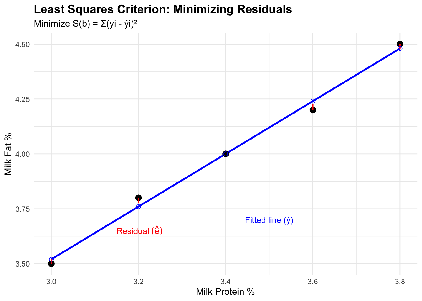
**Visual Illustration of the Least Squares Criterion**
To understand what we're minimizing, let's visualize the residuals (errors) between observed data points and the fitted regression line. The least squares criterion finds the line that minimizes the sum of the squared vertical distances (residuals).
```{r}
#| echo: true
#| fig-width: 7
#| fig-height: 5
library(ggplot2)

# Simple example data: milk fat vs protein
protein <- c(3.0, 3.2, 3.4, 3.6, 3.8)
fat <- c(3.5, 3.8, 4.0, 4.2, 4.5)

# Fit regression
fit <- lm(fat ~ protein)
b0 <- coef(fit)[1]
b1 <- coef(fit)[2]
fitted_values <- predict(fit)
residuals <- residuals(fit)

# Create data frame for plotting
plot_data <- data.frame(
  protein = protein,
  fat = fat,
  fitted = fitted_values,
  residual = residuals
)

# Create visualization
ggplot(plot_data, aes(x = protein, y = fat)) +
  # Regression line
  geom_smooth(method = "lm", se = FALSE, color = "blue", linewidth = 1) +
  # Observed points
  geom_point(size = 3, color = "black") +
  # Residual lines (vertical distances)
  geom_segment(aes(x = protein, xend = protein,
                   y = fat, yend = fitted),
               color = "red", linetype = "dashed", linewidth = 0.8) +
  # Fitted points
  geom_point(aes(y = fitted), color = "blue", size = 2, shape = 1) +
  # Labels
  labs(title = "Least Squares Criterion: Minimizing Residuals",
       subtitle = "Minimize S(b) = Σ(yi - ŷi)²",
       x = "Milk Protein %",
       y = "Milk Fat %") +
  # Annotations
  annotate("text", x = 3.15, y = 3.65,
           label = "Residual~(hat(e))",
           color = "red", size = 3.5, hjust = 0, parse = TRUE) +
  annotate("text", x = 3.5, y = 3.7,
           label = "Fitted line (ŷ)",
           color = "blue", size = 3.5) +
  theme_minimal() +
  theme(plot.title = element_text(face = "bold", size = 14),
        plot.subtitle = element_text(size = 11))
```
The red dashed lines represent the residuals $e_i = y_i - \hat{y}_i$. The least squares method finds the values of $b_0$ and $b_1$ that make the sum of the **squared lengths** of these red lines as small as possible: $SSE = \sum_{i=1}^{n} e_i^2$.
Let's expand this expression:
$$
S(\boldsymbol{b}) = (\boldsymbol{y}' - (\mathbf{X}\boldsymbol{b})')(\boldsymbol{y} - \mathbf{X}\boldsymbol{b})
$$
$$
= (\boldsymbol{y}' - \boldsymbol{b}'\mathbf{X}')(\boldsymbol{y} - \mathbf{X}\boldsymbol{b})
$$
$$
= \boldsymbol{y}'\boldsymbol{y} - \boldsymbol{y}'\mathbf{X}\boldsymbol{b} - \boldsymbol{b}'\mathbf{X}'\boldsymbol{y} + \boldsymbol{b}'\mathbf{X}'\mathbf{X}\boldsymbol{b}
$$
Since $\boldsymbol{b}'\mathbf{X}'\boldsymbol{y}$ is a scalar, its transpose is equal to itself: $(\boldsymbol{b}'\mathbf{X}'\boldsymbol{y})' = \boldsymbol{y}'(\mathbf{X}')'(\boldsymbol{b}')' = \boldsymbol{y}'\mathbf{X}\boldsymbol{b}$. Therefore, the two middle terms are identical.
$$S(\boldsymbol{b}) = \boldsymbol{y}'\boldsymbol{y} - 2\boldsymbol{b}'\mathbf{X}'\boldsymbol{y} + \boldsymbol{b}'\mathbf{X}'\mathbf{X}\boldsymbol{b}$$
### Deriving the Normal Equations
To find the vector $\boldsymbol{b}$ that minimizes this function, we need to take the derivative of $S(\boldsymbol{b})$ with respect to $\boldsymbol{b}$ and set it to zero. Using the rules of matrix calculus:
- $\frac{\partial(\boldsymbol{a}'\boldsymbol{x})}{\partial\boldsymbol{x}} = \boldsymbol{a}$
- $\frac{\partial(\boldsymbol{x}'\mathbf{A}\boldsymbol{x})}{\partial\boldsymbol{x}} = 2\mathbf{A}\boldsymbol{x}$ (for symmetric $\mathbf{A}$)
Applying these rules to $S(\boldsymbol{b})$:
$$ \frac{\partial S(\boldsymbol{b})}{\partial \boldsymbol{b}} = -2\mathbf{X}'\boldsymbol{y} + 2\mathbf{X}'\mathbf{X}\boldsymbol{b} $$
Setting the derivative to a vector of zeros:
$$ -2\mathbf{X}'\boldsymbol{y} + 2\mathbf{X}'\mathbf{X}\boldsymbol{b} = \mathbf{0} $$
$$ \implies \mathbf{X}'\mathbf{X}\boldsymbol{b} = \mathbf{X}'\boldsymbol{y} $$
This fundamental result is the **Normal Equations**. Any vector $\boldsymbol{b}$ that satisfies the normal equations is a least squares estimator of $\boldsymbol{\beta}$. If the matrix $\mathbf{X}'\mathbf{X}$ is full rank (invertible), there is a unique solution:
::: {.callout-important icon=true}
## The Least Squares Solution
When $\mathbf{X}'\mathbf{X}$ is invertible (full rank), the unique least squares estimator is:
$$ \boldsymbol{b} = (\mathbf{X}'\mathbf{X})^{-1}\mathbf{X}'\boldsymbol{y} $$
This is the **fundamental formula** for least squares estimation. It provides the parameter estimates that minimize the sum of squared residuals. Everything we do in linear models—hypothesis testing, confidence intervals, predictions—builds from this solution.
:::
### Properties of Least Squares Estimators
#### 1. Unbiasedness
Under the Gauss-Markov assumption that $E(\boldsymbol{e}) = \mathbf{0}$, the LS estimator $\boldsymbol{b}$ is an unbiased estimator of $\boldsymbol{\beta}$.
**Proof:**
We start with the solution for $\boldsymbol{b}$ and substitute $\boldsymbol{y} = \mathbf{X}\boldsymbol{\beta} + \boldsymbol{e}$.
$$
\begin{aligned}
E(\boldsymbol{b}) &= E[(\mathbf{X}'\mathbf{X})^{-1}\mathbf{X}'\boldsymbol{y}] \\
&= E[(\mathbf{X}'\mathbf{X})^{-1}\mathbf{X}'(\mathbf{X}\boldsymbol{\beta} + \boldsymbol{e})] \\
&= E[(\mathbf{X}'\mathbf{X})^{-1}\mathbf{X}'\mathbf{X}\boldsymbol{\beta} + (\mathbf{X}'\mathbf{X})^{-1}\mathbf{X}'\boldsymbol{e}] \\
&= E[\mathbf{I}\boldsymbol{\beta} + (\mathbf{X}'\mathbf{X})^{-1}\mathbf{X}'\boldsymbol{e}] \\
&= E[\boldsymbol{\beta}] + E[(\mathbf{X}'\mathbf{X})^{-1}\mathbf{X}'\boldsymbol{e}]
\end{aligned}
$$
Since $\mathbf{X}$ and $\boldsymbol{\beta}$ are fixed (not random), $E[\boldsymbol{\beta}] = \boldsymbol{\beta}$. The expectation of the second term is:
$$ E[(\mathbf{X}'\mathbf{X})^{-1}\mathbf{X}'\boldsymbol{e}] = (\mathbf{X}'\mathbf{X})^{-1}\mathbf{X}'E[\boldsymbol{e}] $$
By assumption, $E[\boldsymbol{e}] = \mathbf{0}$. Therefore, the second term is zero.
$$ E(\boldsymbol{b}) = \boldsymbol{\beta} + \mathbf{0} = \boldsymbol{\beta} $$
Thus, the least squares estimator is unbiased. On average, it will equal the true parameter value.
#### 2. Variance of `b`
Under the Gauss-Markov assumptions, $E(\boldsymbol{e})=\mathbf{0}$ and $Var(\boldsymbol{e}) = \sigma^2\mathbf{I}$, we can derive the variance-covariance matrix of the estimator $\boldsymbol{b}$.
**Derivation:**
The variance of a vector $\boldsymbol{b}$ is defined as $Var(\boldsymbol{b}) = E[(\boldsymbol{b} - E(\boldsymbol{b}))(\boldsymbol{b} - E(\boldsymbol{b}))']$.
Since $E(\boldsymbol{b}) = \boldsymbol{\beta}$, we have $\boldsymbol{b} - E(\boldsymbol{b}) = (\mathbf{X}'\mathbf{X})^{-1}\mathbf{X}'\boldsymbol{e}$.
$$
\begin{aligned}
Var(\boldsymbol{b}) &= E[(\boldsymbol{b} - \boldsymbol{\beta})(\boldsymbol{b} - \boldsymbol{\beta})'] \\
&= E[ ((\mathbf{X}'\mathbf{X})^{-1}\mathbf{X}'\boldsymbol{e}) ((\mathbf{X}'\mathbf{X})^{-1}\mathbf{X}'\boldsymbol{e})' ] \\
&= E[ (\mathbf{X}'\mathbf{X})^{-1}\mathbf{X}'\boldsymbol{e} \boldsymbol{e}'\mathbf{X}(\mathbf{X}'\mathbf{X})^{-1} ] \\
&= (\mathbf{X}'\mathbf{X})^{-1}\mathbf{X}' E[\boldsymbol{e}\boldsymbol{e}'] \mathbf{X}(\mathbf{X}'\mathbf{X})^{-1}
\end{aligned}
$$
By definition, $Var(\boldsymbol{e}) = E[\boldsymbol{e}\boldsymbol{e}'] = \sigma^2\mathbf{I}$.
$$
\begin{aligned}
Var(\boldsymbol{b}) &= (\mathbf{X}'\mathbf{X})^{-1}\mathbf{X}' (\sigma^2\mathbf{I}) \mathbf{X}(\mathbf{X}'\mathbf{X})^{-1} \\
&= \sigma^2 (\mathbf{X}'\mathbf{X})^{-1}\mathbf{X}'\mathbf{X}(\mathbf{X}'\mathbf{X})^{-1} \\
&= \sigma^2 (\mathbf{X}'\mathbf{X})^{-1} \mathbf{I} \\
&= \sigma^2 (\mathbf{X}'\mathbf{X})^{-1}
\end{aligned}
$$
::: {.callout-note}
## Notation: What is p?
Throughout this course, **p** denotes the **total number of parameters** in the model, including the intercept. For simple linear regression:
* $\boldsymbol{\beta} = (\beta_0, \beta_1)'$ contains 2 parameters, so **p = 2**
* The design matrix $\mathbf{X}$ has dimensions $n \times p$ (n rows, p columns)
* Degrees of freedom for error: $df = n - p$
In Week 6 (Multiple Regression), we will sometimes write "p-1 predictor variables" to emphasize that one of the p parameters is the intercept, leaving p-1 actual covariates.
:::
::: {.callout-note}
#### Variance-Covariance Matrix of $\boldsymbol{b}$
The variance-covariance matrix of the least squares estimator is:
$$ Var(\boldsymbol{b}) = \sigma^2 (\mathbf{X}'\mathbf{X})^{-1} $$
The diagonal elements of this matrix are the variances of the individual parameter estimates ($Var(b_0), Var(b_1), \dots$), and the off-diagonal elements are the covariances ($Cov(b_i, b_j)$).
:::
### The Gauss-Markov Theorem
This is one of the most important theorems in statistics. It gives us the theoretical justification for using least squares.
::: {.callout-important}
#### The Gauss-Markov Theorem
Under the assumptions of the linear model ($E(\boldsymbol{e}) = \mathbf{0}$, $Var(\boldsymbol{e}) = \sigma^2\mathbf{I}$, and $\mathbf{X}$ is fixed), the least squares estimator $\boldsymbol{b} = (\mathbf{X}'\mathbf{X})^{-1}\mathbf{X}'\boldsymbol{y}$ is the **Best Linear Unbiased Estimator (BLUE)** of $\boldsymbol{\beta}$.
- **Best**: Minimum variance among all linear unbiased estimators.
- **Linear**: It is a linear function of the observations $\boldsymbol{y}$.
- **Unbiased**: $E(\boldsymbol{b}) = \boldsymbol{\beta}$.
:::
The proof is more involved, but it essentially shows that any other linear unbiased estimator has a variance that is at least as large as the variance of the LS estimator.
### Projection Matrices and the Geometry of Least Squares
The geometry of least squares provides a powerful way to visualize what's happening. The key is the **hat matrix**, $\mathbf{H}$.
The vector of fitted values $\hat{\boldsymbol{y}}$ is calculated as:
$$ \hat{\boldsymbol{y}} = \mathbf{X}\boldsymbol{b} = \mathbf{X}(\mathbf{X}'\mathbf{X})^{-1}\mathbf{X}'\boldsymbol{y} $$
Let's define the **Hat Matrix (H)** as:
$$ \mathbf{H} = \mathbf{X}(\mathbf{X}'\mathbf{X})^{-1}\mathbf{X}' $$
So, $\hat{\boldsymbol{y}} = \mathbf{H}\boldsymbol{y}$. The hat matrix "puts the hat on y". It projects the observed data vector $\boldsymbol{y}$ onto the column space of the design matrix $\mathbf{X}$. The fitted values $\hat{\boldsymbol{y}}$ are the shadow that $\boldsymbol{y}$ casts onto the space defined by the model.
**Properties of H:**
1. **Symmetric**: $\mathbf{H}' = \mathbf{H}$
2. **Idempotent**: $\mathbf{H}\mathbf{H} = \mathbf{H}$ (Projecting a projection doesn\'t change anything).
The residual vector can also be expressed using a projection matrix:
$$
\begin{aligned}
\boldsymbol{e} = \boldsymbol{y} - \hat{\boldsymbol{y}} \\
&= \boldsymbol{y} - \mathbf{H}\boldsymbol{y} \\
&= (\mathbf{I} - \mathbf{H})\boldsymbol{y}
\end{aligned}
$$
The matrix $(\mathbf{I} - \mathbf{H})$ is also symmetric and idempotent. It projects $\boldsymbol{y}$ onto the space orthogonal to the column space of $\mathbf{X}$. This is why the residuals are orthogonal to the fitted values: $\hat{\boldsymbol{y}}'\boldsymbol{e} = 0$.
### Sum of Squares Decomposition
The total variation in the data can be partitioned into variation explained by the model and the unexplained (residual) variation.
- **Total Sum of Squares (SST)**: Measures the total variation of y around its mean.
$$ SST = \sum(y_i - \bar{y})^2 = \boldsymbol{y}'\boldsymbol{y} - n\bar{y}^2 $$
- **Model Sum of Squares (SSM)**: Measures the variation explained by the regression model.
$$ SSM = \sum(\hat{y}_i - \bar{y})^2 = \boldsymbol{b}'\mathbf{X}'\boldsymbol{y} - n\bar{y}^2 $$
- **Error Sum of Squares (SSE)**: Measures the unexplained variation.
$$ SSE = \sum(y_i - \hat{y}_i)^2 = \boldsymbol{e}'\boldsymbol{e} = \boldsymbol{y}'\boldsymbol{y} - \boldsymbol{b}'\mathbf{X}'\boldsymbol{y} $$
A fundamental identity is:
$$ SST = SSM + SSE $$
### Variance Estimation
Our $Var(\boldsymbol{b})$ formula depends on the unknown population parameter $\sigma^2$. We must estimate it from the data. The estimator for $\sigma^2$ is the **Mean Square Error (MSE)**.
$$ \hat{\sigma}^2 = MSE = \frac{SSE}{n-p} $$
Where:
- $n$ = number of observations
- $p$ = number of parameters in $\boldsymbol{\beta}$ (including the intercept), which is equal to the rank of $\mathbf{X}$.
The quantity $(n-p)$ is the degrees of freedom for error. We can show that $E(MSE) = \sigma^2$, so it is an unbiased estimator.
With this, we can estimate the variance-covariance matrix of $\boldsymbol{b}$:
$$ \widehat{Var}(\boldsymbol{b}) = \hat{\sigma}^2 (\mathbf{X}'\mathbf{X})^{-1} $$
The standard error of an individual estimate $b_j$ is the square root of the $j$-th diagonal element of this matrix.
### Distribution Theory (Under Normality Assumption)
If we add the assumption that the errors are normally distributed, $\boldsymbol{e} \sim N(\mathbf{0}, \sigma^2\mathbf{I})$, we can derive the distributions of our estimators, which is essential for hypothesis testing.
- $�oldsymbol{y} \sim N(\mathbf{X}\boldsymbol{\beta}, \sigma^2\mathbf{I})$
- $�oldsymbol{b} \sim N(\boldsymbol{\beta}, \sigma^2(\mathbf{X}'\mathbf{X})^{-1})$
- $�rac{SSE}{\sigma^2} \sim \chi^2_{n-p}$ (Chi-squared distribution with $n-p$ degrees of freedom)
- $�oldsymbol{b}$ and $SSE$ are statistically independent.
These results lead directly to the t-tests for individual coefficients and the F-test for the overall model, which we will use extensively.
---
## Small Numerical Example
Let's analyze the relationship between milk protein percentage (x) and milk fat percentage (y) in a sample of 5 dairy cows.
| Protein % (x) | Fat % (y) |
|:-------------:|
| 3.0 | 3.5 |
| 3.2 | 3.8 |
| 3.4 | 4.0 |
| 3.6 | 4.2 |
| 3.8 | 4.5 |
The model is $y_i = \beta_0 + \beta_1 x_i + e_i$.
**1. Construct Matrices**
$$ \boldsymbol{y} = \begin{pmatrix} 3.5 \\ 3.8 \\ 4.0 \\ 4.2 \\ 4.5 \end{pmatrix}, \quad \mathbf{X} = \begin{pmatrix} 1 & 3.0 \\ 1 & 3.2 \\ 1 & 3.4 \\ 1 & 3.6 \\ 1 & 3.8 \end{pmatrix} $$
**2. Calculate $\mathbf{X}'\mathbf{X}$ and $\mathbf{X}'\boldsymbol{y}$**
$$ \mathbf{X}'\mathbf{X} = \begin{pmatrix} 1 & 1 & 1 & 1 & 1 \\ 3.0 & 3.2 & 3.4 & 3.6 & 3.8 \end{pmatrix} \begin{pmatrix} 1 & 3.0 \\ 1 & 3.2 \\ 1 & 3.4 \\ 1 & 3.6 \\ 1 & 3.8 \end{pmatrix} = \begin{pmatrix} 5 & 17.0 \\ 17.0 & 58.6 \end{pmatrix} $$
$$ \mathbf{X}'\boldsymbol{y} = \begin{pmatrix} 1 & 1 & 1 & 1 & 1 \\ 3.0 & 3.2 & 3.4 & 3.6 & 3.8 \end{pmatrix} \begin{pmatrix} 3.5 \\ 3.8 \\ 4.0 \\ 4.2 \\ 4.5 \end{pmatrix} = \begin{pmatrix} 20.0 \\ 68.34 \end{pmatrix} $$
**3. Find the Inverse $(\mathbf{X}'\mathbf{X})^{-1}$**
The determinant is $det(\mathbf{X}'\mathbf{X}) = (5)(58.6) - (17.0)(17.0) = 293 - 289 = 4$.
The inverse is:
$$ (\mathbf{X}'\mathbf{X})^{-1} = \frac{1}{4} \begin{pmatrix} 58.6 & -17.0 \\ -17.0 & 5 \end{pmatrix} = \begin{pmatrix} 14.65 & -4.25 \\ -4.25 & 1.25 \end{pmatrix} $$
**4. Solve for $\boldsymbol{b}$**
$$ \boldsymbol{b} = (\mathbf{X}'\mathbf{X})^{-1}\mathbf{X}'\boldsymbol{y} = \begin{pmatrix} 14.65 & -4.25 \\ -4.25 & 1.25 \end{pmatrix} \begin{pmatrix} 20.0 \\ 68.34 \end{pmatrix} = \begin{pmatrix} 293 - 290.445 \\ -85 + 85.425 \end{pmatrix} = \begin{pmatrix} 2.555 \\ 0.425 \end{pmatrix} $$
So, $b_0 = 2.555$ and $b_1 = 0.425$. The fitted equation is $\hat{y} = 2.555 + 0.425x$.
**5. Decompose Sums of Squares**
First, find $\boldsymbol{b}'\mathbf{X}'\boldsymbol{y}$:
$$ \boldsymbol{b}'\mathbf{X}'\boldsymbol{y} = \begin{pmatrix} 2.555 & 0.425 \end{pmatrix} \begin{pmatrix} 20.0 \\ 68.34 \end{pmatrix} = 51.1 + 29.0445 = 80.1445 $$
And $\boldsymbol{y}'\boldsymbol{y}$:
$$ \boldsymbol{y}'\boldsymbol{y} = 3.5^2 + 3.8^2 + 4.0^2 + 4.2^2 + 4.5^2 = 12.25 + 14.44 + 16.0 + 17.64 + 20.25 = 80.58 $$
The mean of y is $\bar{y} = 20.0 / 5 = 4.0$.
- $SSE = \boldsymbol{y}'\boldsymbol{y} - \boldsymbol{b}'\mathbf{X}'\boldsymbol{y} = 80.58 - 80.1445 = 0.4355$
- $SST = \boldsymbol{y}'\boldsymbol{y} - n\bar{y}^2 = 80.58 - 5(4.0)^2 = 80.58 - 80 = 0.58$
- $SSM = SST - SSE = 0.58 - 0.4355 = 0.1445$
**6. Estimate Variance and Construct Confidence Intervals**
Here, $n=5$ and $p=2$.
$$ \hat{\sigma}^2 = MSE = \frac{SSE}{n-p} = \frac{0.4355}{5-2} = 0.145167 $$
Now find the estimated variance of $\boldsymbol{b}$:
$$ \widehat{Var}(\boldsymbol{b}) = \hat{\sigma}^2 (\mathbf{X}'\mathbf{X})^{-1} = 0.145167 \begin{pmatrix} 14.65 & -4.25 \\ -4.25 & 1.25 \end{pmatrix} = \begin{pmatrix} 2.1267 & -0.6169 \\ -0.6169 & 0.1815 \end{pmatrix} $$
So, $\widehat{Var}(b_1) = 0.1815$, and the standard error is $se(b_1) = \sqrt{0.1815} = 0.426$.
Let's construct a 95% confidence interval for $\beta_1$. The critical t-value for $df = n-p=3$ is $t_{0.025, 3} = 3.182$.
$$ CI = b_1 \pm t_{0.025, 3} \times se(b_1) = 0.425 \pm 3.182 \times 0.426 = 0.425 \pm 1.355 $$
CI = (-0.93, 1.78). Since this interval contains 0, we cannot conclude that there is a significant linear relationship between milk protein and fat percentage in this very small sample.
---
## Realistic Livestock Application
**Scenario**: We want to predict the weaning weight of lambs based on their birth weight. We have data from 40 lambs from a research flock.
**Objective**: Fit a simple linear regression, compute the full ANOVA table, and test the significance of the regression.
First, let's load and view a sample of the data.
````{r}
#| echo: true
lamb_data <- read.csv("data/lamb_data.csv")
head(lamb_data)
````
We fit the model: `Wean_Weight_kg` = $\beta_0 + \beta_1$`Birth_Weight_kg` + $e$.
We will perform the calculations manually using matrix algebra in R, then construct the ANOVA table.
````{r}
#| echo: true
# Matrix calculations
y <- lamb_data$Wean_Weight_kg
x <- lamb_data$Birth_Weight_kg
n <- length(y)
X <- cbind(1, x)

# Solve normal equations
XtX <- t(X) %*% X
Xty <- t(X) %*% y
b <- solve(XtX) %*% Xty

# Sum of Squares
ybar <- mean(y)
b_Xty <- t(b) %*% Xty
yty <- t(y) %*% y

SST <- yty - n * ybar^2
SSE <- yty - b_Xty
SSM <- SST - SSE

# ANOVA Table components
p <- 2 # number of parameters
df_M <- p - 1
df_E <- n - p
df_T <- n - 1

MSM <- SSM / df_M
MSE <- SSE / df_E
F_stat <- MSM / MSE

# Print results
cat("Parameter Estimates (b0, b1):\n")
print(b)
cat("\n--- ANOVA Table ---\n")
cat(sprintf("% -10s %4s %8s %8s %8s\n", "Source", "df", "SS", "MS", "F"))
cat(sprintf("% -10s %4d %8.2f %8.2f %8.2f\n", "Model", df_M, SSM, MSM, F_stat))
cat(sprintf("% -10s %4d %8.2f %8.2f\n", "Error", df_E, SSE, MSE))
cat(sprintf("% -10s %4d %8.2f\n", "Total", df_T, SST))
````
**Interpretation**:
The F-statistic is very large (215.11). The critical F-value for 1 and 38 degrees of freedom at $\alpha=0.05$ is approximately 4.10. Since our calculated F-statistic is much larger, we reject the null hypothesis $H_0: \beta_1 = 0$. There is a highly significant linear relationship between birth weight and weaning weight in these lambs. The model explains a large proportion of the total variation in weaning weight.
---
## Solver Implementation in R
Let's implement the core theoretical concepts from this week in R and verify their properties. We will use the small dairy cow data example.
````{r}
#| echo: true
# Data from the small example
y <- c(3.5, 3.8, 4.0, 4.2, 4.5)
x <- c(3.0, 3.2, 3.4, 3.6, 3.8)
n <- length(y)
p <- 2

# Design Matrix
X <- cbind(1, x)

# 1. Hat Matrix (H) and Projection
H <- X %*% solve(t(X) %*% X) %*% t(X)
cat("Hat Matrix H:\n")
print(round(H, 3))
# Verify properties of H
# H should be symmetric
is_symmetric <- all.equal(H, t(H))
cat("\nIs H symmetric? ", is_symmetric, "\n")
# H should be idempotent (H*H = H)
H_squared <- H %*% H
is_idempotent <- all.equal(H, H_squared)
cat("Is H idempotent? ", is_idempotent, "\n")
# 2. Get fitted values and residuals using H
y_hat <- H %*% y
residuals <- (diag(n) - H) %*% y

cat("\nFitted values (y_hat):\n")
print(y_hat)
cat("\nResiduals (e):\n")
print(residuals)
# Verify that residuals are orthogonal to fitted values
orthogonality_check <- t(y_hat) %*% residuals
cat("\nInner product of y_hat and e (should be ~0): ", orthogonality_check, "\n")
# 3. Sum of Squares calculation
# Using matrix formulas
b <- solve(t(X)%*%X) %*% t(X)%*%y
SST_mat <- t(y) %*% y - n * mean(y)^2
SSE_mat <- t(y) %*% y - t(b) %*% t(X) %*% y
SSM_mat <- t(b) %*% t(X) %*% y - n * mean(y)^2

cat("\n--- Sum of Squares ---\n")
cat("SST: ", SST_mat, "\n")
cat("SSM: ", SSM_mat, "\n")
cat("SSE: ", SSE_mat, "\n")
cat("SSM + SSE: ", SSM_mat + SSE_mat, "\n")
# 4. Variance Estimation
sigma2_hat <- SSE_mat / (n - p)
cat("\nEstimated Residual Variance (sigma^2): ", c(sigma2_hat), "\n")
# Variance-Covariance matrix of b
var_b <- solve(t(X) %*% X) * c(sigma2_hat)
cat("\nVariance-Covariance Matrix of b:\n")
print(var_b)
# Standard error of b1
se_b1 <- sqrt(var_b[2, 2])
cat("\nStandard Error of b1: ", se_b1, "\n")
# 5. Compare with lm() output
fit <- lm(y ~ x)
summary(fit)
````
As you can see, our manually calculated values for the estimates, standard errors, residual variance ($\hat{\sigma}^2$, called "Residual standard error" squared in the `lm` summary), and sums of squares all match the output from R's built-in `lm()` function. This confirms our understanding of the underlying theory.
**Previous**: [Week 4: Simple Linear Regression](../Week04_SimpleRegression/Week04_SimpleRegression.qmd)
**Next**: [Week 6: Multiple Regression](../Week06_MultipleRegression/Week06_MultipleRegression.qmd)