---
title: "Week 12: Unequal Subclass Numbers & Non-Full Rank Models"
format:
html:
toc: true
toc-depth: 3
number-sections: true
code-fold: false
code-tools: true
bibliography: ../references.bib
---
::: {.callout-note icon=false}
## Learning Objectives
By the end of this week, you will be able to:
1. **Understand** the consequences of **unbalanced data** on **design matrix rank** and the resulting impact on **parameter estimation**
2. **Compute** and **use** **generalized inverses** to solve **normal equations** when $\mathbf{X}'\mathbf{X}$ is singular
3. **Determine** which **linear functions of parameters** are **estimable** in **rank-deficient models** using the **row space criterion**
4. **Apply** **constraints** (set-to-zero, sum-to-zero) to obtain **unique parameter solutions** and interpret their effects
5. **Analyze** realistic **multi-farm livestock datasets** with **missing cells** using appropriate methods (**Type III SS**, **estimable contrasts**, `emmeans`)
:::
---
## Introduction: When Real Data Gets Messy
In Weeks 7 and 8, we worked primarily with balanced designs where every group had equal sample sizes. The mathematics was clean: $\mathbf{X}'\mathbf{X}$ was full rank, orthogonal contrasts partitioned sums of squares neatly, and every parameter was uniquely estimable. Real livestock data is rarely so cooperative.
Consider these common scenarios in animal breeding and genetics:
- **Sire evaluation**: Some bulls have 3 progeny records, others have 500. Dairy genetic evaluations routinely handle sires with vastly different progeny group sizes.
- **Multi-farm breed comparisons**: Not all breeds are raised on all farms. A Charolais breeder in Texas may not also raise Holsteins.
- **Longitudinal studies**: Animal mortality and dropout create unbalanced groups. A 24-month feeding trial that starts with equal groups rarely ends that way.
- **Commercial records**: Observational data from commercial operations is inherently unbalanced. Farmers make decisions—culling, treatment, grouping—that create inequality.
When data is unbalanced, three critical things happen:
1. **$\mathbf{X}'\mathbf{X}$ may not be full rank** → The normal equations have infinitely many solutions
2. **Type I, II, and III sums of squares differ** → The order of fitting effects matters
3. **Individual parameters may not be estimable** → But contrasts (differences) often are
This week, we confront the reality of unbalanced data head-on. We'll learn:
- Why rank deficiency occurs and what it means
- How to solve singular systems using generalized inverses
- Which functions are estimable and which are not
- How to use constraints to get unique solutions
- Practical methods for analyzing real unbalanced datasets
::: {.callout-important}
### Why This Week Matters in Animal Breeding
In real animal breeding programs:
- **Sires have 3 to 500+ progeny** (progeny test designs are highly unbalanced)
- **Contemporary groups vary** from 5 to 200 animals
- **Some breed × environment combinations never occur** (climate, management, economics)
- **Missing data is the norm**, not the exception
Understanding rank deficiency and estimability is not academic—it's essential for genetic evaluation, breed comparisons, and making sound breeding decisions from messy commercial data.
:::
::: {.callout-note}
### Connection to Previous Weeks
This week synthesizes concepts from:
- **Week 2**: Generalized inverses (now we use them!)
- **Week 7**: Cell means vs. effects models (now unbalanced)
- **Week 8**: Estimable functions and contrasts (critical when rank deficient)
- **Week 10**: Type I/II/III sums of squares (essential for unbalanced ANOVA)
Week 12 is where all these pieces unite to handle real-world complexity.
:::
### Chapter Roadmap
Here's what we'll cover:
1. **Mathematical Theory** (Sections 2-5): Rank deficiency, generalized inverses, estimability, constraints
2. **Small Example** (Section 6): Sheep fleece weight by breed (n=3,2,1) – hand-calculable
3. **R Implementation** (Section 7): Building solvers that handle singular systems
4. **Realistic Application** (Section 8): Multi-farm beef cattle with missing cells (n=177)
5. **Practical Guidelines** (Section 9): What to do when you encounter unbalanced data
By the end, you'll be equipped to handle the messy reality of livestock data with confidence.
---
## Mathematical Theory of Rank Deficiency
### Rank Deficiency in Linear Models
Recall the **effects model** for one-way ANOVA:
$$
y_{ij} = \mu + \alpha_i + e_{ij}
$$ {#eq-effects-model}
where:
- $y_{ij}$: observation $j$ in group $i$ (scalar)
- $\mu$: overall mean (scalar parameter)
- $\alpha_i$: effect of group $i$ (scalar parameter, $i = 1, \ldots, g$)
- $e_{ij}$: random error, $e_{ij} \sim N(0, \sigma^2)$
In matrix form:
$$
\mathbf{y} = \mathbf{X}\boldsymbol{\beta} + \mathbf{e}
$$ {#eq-matrix-form}
where:
- $\mathbf{y}$: $n \times 1$ response vector
- $\mathbf{X}$: $n \times (g+1)$ design matrix
- $\boldsymbol{\beta} = [\mu, \alpha_1, \alpha_2, \ldots, \alpha_g]'$: $(g+1) \times 1$ parameter vector
- $\mathbf{e}$: $n \times 1$ error vector
For a 3-group study with $n_1=3, n_2=2, n_3=1$ observations:
$$
\mathbf{X} = \begin{bmatrix}
1 & 1 & 0 & 0 \\
1 & 1 & 0 & 0 \\
1 & 1 & 0 & 0 \\
1 & 0 & 1 & 0 \\
1 & 0 & 1 & 0 \\
1 & 0 & 0 & 1
\end{bmatrix}_{6 \times 4}
$$ {#eq-design-matrix-effects}
**The problem**: Column 1 (intercept) equals the sum of columns 2, 3, and 4:
$$
\text{Column 1} = \text{Column 2} + \text{Column 3} + \text{Column 4}
$$
Therefore: $r(\mathbf{X}) = 3 < 4 = p$ (number of parameters)
The design matrix **does not have full column rank**. This is not a numerical precision issue—it's structural. The model has **inherent redundancy**: we cannot simultaneously estimate both $\mu$ and all $\alpha_i$ because they are **confounded**.
::: {.callout-warning}
### Rank Deficiency is Structural, Not Numerical
This is not computational roundoff error. The model
$$y_{ij} = \mu + \alpha_i + e_{ij}$$
has **inherent redundancy**:
- We cannot estimate both $\mu$ and all $\alpha_i$ uniquely
- The intercept and group effects are **confounded**
- For any solution, we can add a constant to $\mu$ and subtract it from all $\alpha_i$—the fit doesn't change
This requires either:
1. Using a different parameterization (cell means model)
2. Imposing constraints to remove redundancy
3. Focusing only on estimable functions (contrasts)
:::
### Consequences for the Normal Equations
When $r(\mathbf{X}'\mathbf{X}) < p$, the normal equations
$$
\mathbf{X}'\mathbf{X}\mathbf{b} = \mathbf{X}'\mathbf{y}
$$ {#eq-normal-equations}
have the following properties:
1. **$\mathbf{X}'\mathbf{X}$ is singular** (not invertible): $\det(\mathbf{X}'\mathbf{X}) = 0$
2. **$(\mathbf{X}'\mathbf{X})^{-1}$ does not exist**: The regular inverse is undefined
3. **Infinitely many solutions exist**: Any $\mathbf{b}$ satisfying $\mathbf{X}'\mathbf{X}\mathbf{b} = \mathbf{X}'\mathbf{y}$ is a solution
4. **Individual parameter estimates are NOT unique**: Different solution methods give different $\mathbf{b}$
However—and this is critical:
5. **Fitted values $\hat{\mathbf{y}} = \mathbf{Xb}$ are unique**: All solutions give the same $\hat{\mathbf{y}}$
6. **Residuals $\mathbf{e} = \mathbf{y} - \hat{\mathbf{y}}$ are unique**: All solutions give the same residuals
7. **SSE is unique**: $SSE = \mathbf{e}'\mathbf{e}$ is the same for all solutions
8. **Estimable functions $\mathbf{c}'\boldsymbol{\beta}$ are unique**: If $\mathbf{c}'\boldsymbol{\beta}$ is estimable, $\mathbf{c}'\mathbf{b}$ is the same for all solutions
### Algebraic Proof of Uniqueness
**Claim**: For any two solutions $\mathbf{b}_1$ and $\mathbf{b}_2$ to the normal equations, $\mathbf{Xb}_1 = \mathbf{Xb}_2$.
**Proof**:
Both satisfy the normal equations:
$$
\mathbf{X}'\mathbf{X}\mathbf{b}_1 = \mathbf{X}'\mathbf{y} \quad \text{and} \quad \mathbf{X}'\mathbf{X}\mathbf{b}_2 = \mathbf{X}'\mathbf{y}
$$
Subtracting:
$$
\mathbf{X}'\mathbf{X}(\mathbf{b}_1 - \mathbf{b}_2) = \mathbf{0}
$$
Premultiplying by $(\mathbf{b}_1 - \mathbf{b}_2)'$:
$$
(\mathbf{b}_1 - \mathbf{b}_2)'\mathbf{X}'\mathbf{X}(\mathbf{b}_1 - \mathbf{b}_2) = 0
$$
But $\mathbf{X}'\mathbf{X}$ is positive semidefinite, so:
$$
[\mathbf{X}(\mathbf{b}_1 - \mathbf{b}_2)]'[\mathbf{X}(\mathbf{b}_1 - \mathbf{b}_2)] = 0
$$
This implies:
$$
\mathbf{X}(\mathbf{b}_1 - \mathbf{b}_2) = \mathbf{0}
$$
Therefore:
$$
\mathbf{Xb}_1 = \mathbf{Xb}_2
$$
**Conclusion**: Even though $\mathbf{b}_1 \neq \mathbf{b}_2$, the fitted values are identical. $\square$
---
### Generalized Inverses
Since $(\mathbf{X}'\mathbf{X})^{-1}$ doesn't exist when $\mathbf{X}'\mathbf{X}$ is singular, we need an alternative: the **generalized inverse**.
#### Definition
A matrix $\mathbf{G}$ is a **generalized inverse** of $\mathbf{A}$ (denoted $\mathbf{A}^-$) if:
$$
\mathbf{A}\mathbf{A}^-\mathbf{A} = \mathbf{A}
$$ {#eq-ginv-definition}
This is the minimum requirement for a generalized inverse (also called a **reflexive g-inverse**).
**Properties**:
1. **Not unique** for singular matrices: Many matrices satisfy @eq-ginv-definition
2. **Reduces to regular inverse** when $\mathbf{A}$ is nonsingular: If $\mathbf{A}$ is full rank, $\mathbf{A}^- = \mathbf{A}^{-1}$
3. **Provides a solution** to consistent systems: If $\mathbf{Ab} = \mathbf{c}$ is consistent, then $\mathbf{b} = \mathbf{A}^-\mathbf{c}$ is a solution
### Using G-Inverse to Solve Normal Equations
For $\mathbf{X}'\mathbf{X}\mathbf{b} = \mathbf{X}'\mathbf{y}$, any solution has the form:
$$
\mathbf{b} = (\mathbf{X}'\mathbf{X})^-\mathbf{X}'\mathbf{y}
$$ {#eq-ginv-solution}
where $(\mathbf{X}'\mathbf{X})^-$ is any generalized inverse of $\mathbf{X}'\mathbf{X}$.
**Key verification**:
$$
\mathbf{X}'\mathbf{X}\mathbf{b} = \mathbf{X}'\mathbf{X}[(\mathbf{X}'\mathbf{X})^-\mathbf{X}'\mathbf{y}] = \mathbf{X}'\mathbf{y} \quad \checkmark
$$
(using $\mathbf{A}\mathbf{A}^-\mathbf{A} = \mathbf{A}$ with $\mathbf{A} = \mathbf{X}'$)
::: {.callout-important}
### G-Inverse in Solving Normal Equations
For rank-deficient normal equations $\mathbf{X}'\mathbf{X}\mathbf{b} = \mathbf{X}'\mathbf{y}$:
$$
\mathbf{b} = (\mathbf{X}'\mathbf{X})^-\mathbf{X}'\mathbf{y}
$$
**Critical insights**:
1. Different choices of $(\mathbf{X}'\mathbf{X})^-$ give **different $\mathbf{b}$**
2. But **$\mathbf{Xb}$ is always the same** (fitted values unique)
3. **Estimable functions $\mathbf{c}'\mathbf{b}$ are always the same** (if $\mathbf{c}'\boldsymbol{\beta}$ is estimable)
4. Non-estimable functions $\mathbf{c}'\mathbf{b}$ **depend on which $(\mathbf{X}'\mathbf{X})^-$ you use**
In practice: Use any g-inverse for computation, but **only interpret estimable functions**.
:::
### The Moore-Penrose Pseudoinverse
Among all generalized inverses, one is special: the **Moore-Penrose pseudoinverse** (denoted $\mathbf{A}^+$).
It's the unique matrix satisfying four properties:
1. $\mathbf{A}\mathbf{A}^+\mathbf{A} = \mathbf{A}$ (reflexive)
2. $\mathbf{A}^+\mathbf{A}\mathbf{A}^+ = \mathbf{A}^+$ (minimum norm)
3. $(\mathbf{A}\mathbf{A}^+)' = \mathbf{A}\mathbf{A}^+$ (symmetric)
4. $(\mathbf{A}^+\mathbf{A})' = \mathbf{A}^+\mathbf{A}$ (symmetric)
**Uniqueness**: Only one matrix satisfies all four properties.
**Computation via SVD**: If $\mathbf{A} = \mathbf{U}\mathbf{D}\mathbf{V}'$ (singular value decomposition), then:
$$
\mathbf{A}^+ = \mathbf{V}\mathbf{D}^+\mathbf{U}'
$$
where $\mathbf{D}^+$ replaces each nonzero singular value $d_i$ with $1/d_i$.
**In R**: Use `MASS::ginv(A)` which computes the Moore-Penrose inverse.
::: {.callout-tip}
### Computing G-Inverses in R
```r
library(MASS)

# Compute Moore-Penrose inverse
A_ginv <- ginv(A)

# Verify the property AA⁻A = A
max(abs(A %*% A_ginv %*% A - A))  # Should be ≈ 0 (numerical precision)

# Solve normal equations
XtX <- t(X) %*% X
Xty <- t(X) %*% y
b <- ginv(XtX) %*% Xty
```
**Note**: Any g-inverse works for solving normal equations. `ginv()` is convenient and gives the minimum-norm solution.
:::
---
## Estimability Revisited
In Week 8, we introduced estimable functions for balanced designs. With unbalanced data and rank deficiency, estimability becomes critical.
### Formal Definition
A linear function $\mathbf{c}'\boldsymbol{\beta}$ is **estimable** if and only if:
$$
\mathbf{c}' = \mathbf{a}'\mathbf{X} \quad \text{for some vector } \mathbf{a}
$$ {#eq-estimability-criterion}
**Equivalently**: $\mathbf{c}$ is in the **row space of $\mathbf{X}$**.
**Intuition**: Estimable functions are those that can be expressed as linear combinations of the rows of $\mathbf{X}$—i.e., they're "built into" the design.
### Critical Theorem on Estimability
**Theorem**: If $\mathbf{c}'\boldsymbol{\beta}$ is estimable, then:
1. **$\mathbf{c}'\mathbf{b}$ is unique** (independent of which $(\mathbf{X}'\mathbf{X})^-$ is used)
2. **$\text{Var}(\mathbf{c}'\mathbf{b}) = \mathbf{c}'(\mathbf{X}'\mathbf{X})^-\mathbf{c} \sigma^2$ is unique**
3. **$\mathbf{c}'\mathbf{b}$ is BLUE** of $\mathbf{c}'\boldsymbol{\beta}$ (Best Linear Unbiased Estimator)
**Proof sketch**:
For any two g-inverses $\mathbf{G}_1$ and $\mathbf{G}_2$ of $\mathbf{X}'\mathbf{X}$:
- Solutions: $\mathbf{b}_1 = \mathbf{G}_1\mathbf{X}'\mathbf{y}$ and $\mathbf{b}_2 = \mathbf{G}_2\mathbf{X}'\mathbf{y}$
- If $\mathbf{c}'\boldsymbol{\beta}$ estimable: $\mathbf{c}' = \mathbf{a}'\mathbf{X}$
- Then: $\mathbf{c}'\mathbf{b}_1 = \mathbf{a}'\mathbf{X}\mathbf{b}_1 = \mathbf{a}'\hat{\mathbf{y}}$
- And: $\mathbf{c}'\mathbf{b}_2 = \mathbf{a}'\mathbf{X}\mathbf{b}_2 = \mathbf{a}'\hat{\mathbf{y}}$
- Since $\hat{\mathbf{y}} = \mathbf{Xb}$ is unique, $\mathbf{c}'\mathbf{b}_1 = \mathbf{c}'\mathbf{b}_2$ $\square$
::: {.callout-important}
### Testing Estimability in R
```r
is_estimable <- function(c, X, tol = 1e-10) {
  # Test if c'β is estimable
  # c'β estimable ⟺ c in row space of X
  # ⟺ (X'X)⁻c in column space of X'X
  # ⟺ (X'X)(X'X)⁻c = c

  XtX <- t(X) %*% X
  XtX_ginv <- ginv(XtX)
  projection <- XtX %*% XtX_ginv %*% c

  all(abs(projection - c) < tol)
}

# Example usage
c1 <- c(0, 1, -1, 0)  # α₁ - α₂
is_estimable(c1, X)   # TRUE

c2 <- c(1, 0, 0, 0)   # μ
is_estimable(c2, X)   # FALSE
```
This function checks the criterion: $\mathbf{c}'\boldsymbol{\beta}$ is estimable iff $(\mathbf{X}'\mathbf{X})(\mathbf{X}'\mathbf{X})^-\mathbf{c} = \mathbf{c}$.
:::
### Examples: Estimable vs. Non-Estimable
For the effects model $y_{ij} = \mu + \alpha_i + e_{ij}$ with 3 groups:
**Non-Estimable**:
- $\mu$ (overall mean): Confounded with $\alpha_i$
- $\alpha_1$ (group 1 effect): Not uniquely defined
- Individual $\alpha_i$ values
**Estimable**:
- $\alpha_1 - \alpha_2$ (difference between groups 1 and 2)
- $\alpha_1 - \alpha_3$ (difference between groups 1 and 3)
- $(\alpha_1 + \alpha_2)/2 - \alpha_3$ (average of groups 1,2 vs. group 3)
- Any contrast $\sum c_i \alpha_i$ where $\sum c_i = 0$
- Group means $\mu_i = \mu + \alpha_i$ (these are what we observe!)
**General rule**: In the effects model with rank deficiency:
- Individual $\mu$ and $\alpha_i$ are **not** estimable
- Contrasts $\sum c_i \alpha_i$ with $\sum c_i = 0$ **are** estimable
- Group means $\mu_i = \mu + \alpha_i$ **are** estimable
---
## Constraints for Identifiability
We've seen that rank deficiency leads to non-unique parameter estimates. One way to resolve this: **impose constraints** that remove the redundancy.
### Common Constraint Types
**1. Set-to-zero constraints** (reference cell coding):
Set one parameter to zero, e.g., $\alpha_g = 0$.
- Interpretation: Other $\alpha_i$ are deviations from group $g$
- R default: `lm()` uses this with first level as reference
**2. Sum-to-zero constraints**:
$$\sum_{i=1}^g \alpha_i = 0$$ {#eq-sum-to-zero}
- Interpretation: $\alpha_i$ are deviations from overall mean
- More symmetric than set-to-zero
- Useful for balanced designs
**3. Weighted sum-to-zero constraints**:
$$\sum_{i=1}^g n_i \alpha_i = 0$$ {#eq-weighted-sum}
- Accounts for unequal group sizes
- Each group weighted by sample size
::: {.callout-note}
### Constraints vs. G-Inverses: Two Paths, Same Destination
Two equivalent approaches to handle rank deficiency:
**Approach 1**: Use constraints to achieve full rank
- Augment normal equations with constraint rows
- Solve augmented system for unique $\mathbf{b}$
**Approach 2**: Use g-inverse, focus on estimable functions
- Solve $\mathbf{b} = (\mathbf{X}'\mathbf{X})^-\mathbf{X}'\mathbf{y}$ for any solution
- Only interpret estimable $\mathbf{c}'\mathbf{b}$
**Which to use?**
- Constraints: Good when you want specific parameterization
- G-inverse: Good when you only care about contrasts
**Important**: Choice is computational/interpretational, **not statistical**. Estimable functions $\mathbf{c}'\mathbf{b}$ are the same either way.
:::
---
## Small Example: Sheep Fleece Weight
Let's work through a complete example small enough for hand calculations but rich enough to illustrate all concepts.
### Problem Setup
**Research question**: Compare fleece weight (kg) across three sheep breeds.
**Data** (unbalanced):
| Breed | Fleece Weight (kg) | Sample Size |
|-------|-------------------|-------------|
| Romney | 5.2, 5.4, 5.3 | $n_1 = 3$ |
| Merino | 4.8, 5.0 | $n_2 = 2$ |
| Corriedale | 5.6 | $n_3 = 1$ |
**Total**: $n = 6$ observations
**Note the unbalanced design**: Group sizes are 3, 2, and 1. This is realistic—perhaps Corriedale is a less common breed in the study region.
::: {.callout-note}
### Why This Example?
This example is pedagogically ideal:
- **Small enough** for complete hand calculations
- **Unbalanced** (3, 2, 1) shows rank deficiency clearly
- **Realistic**: Breed comparison with unequal representation
- Demonstrates both **cell means** (full rank) and **effects** (rank deficient) models
- Illustrates **estimability**: What can and can't be uniquely estimated
:::
---
### Cell Means Model (Full Rank)
**Model**:
$$y_{ij} = \mu_i + e_{ij}$$
where $\mu_i$ is the mean for breed $i$ (no overall $\mu$, no $\alpha_i$).
#### Step 1: Design Matrix
$$
\mathbf{X} = \begin{bmatrix}
1 & 0 & 0 \\
1 & 0 & 0 \\
1 & 0 & 0 \\
0 & 1 & 0 \\
0 & 1 & 0 \\
0 & 0 & 1
\end{bmatrix}_{6 \times 3}, \quad
\boldsymbol{\beta} = \begin{bmatrix}
\mu_1 \\
\mu_2 \\
\mu_3
\end{bmatrix}
$$
**Check rank**: $r(\mathbf{X}) = 3 = p$ → **Full rank!**
The cell means model is **always full rank**, even with unbalanced data.
#### Step 2: Normal Equations
$$
\mathbf{X}'\mathbf{X} = \begin{bmatrix}
3 & 0 & 0 \\
0 & 2 & 0 \\
0 & 0 & 1
\end{bmatrix}, \quad
\mathbf{X}'\mathbf{y} = \begin{bmatrix}
15.9 \\
9.8 \\
5.6
\end{bmatrix}
$$
**Note**: $\mathbf{X}'\mathbf{X}$ is **diagonal** (always true for cell means, even unbalanced).
#### Step 3: Solve
Since $\mathbf{X}'\mathbf{X}$ is diagonal and invertible:
$$
(\mathbf{X}'\mathbf{X})^{-1} = \begin{bmatrix}
1/3 & 0 & 0 \\
0 & 1/2 & 0 \\
0 & 0 & 1
\end{bmatrix}
$$
Solution:
$$
\mathbf{b} = (\mathbf{X}'\mathbf{X})^{-1}\mathbf{X}'\mathbf{y} = \begin{bmatrix}
15.9/3 \\
9.8/2 \\
5.6/1
\end{bmatrix} = \begin{bmatrix}
5.30 \\
4.90 \\
5.60
\end{bmatrix}
$$
**Interpretation**:
- $\hat{\mu}_1 = 5.30$ kg (Romney mean)
- $\hat{\mu}_2 = 4.90$ kg (Merino mean)
- $\hat{\mu}_3 = 5.60$ kg (Corriedale mean)
**These are just the group means!** The cell means model directly estimates what we observe.
#### Step 4: Residuals and SSE
Fitted values:
$$
\hat{\mathbf{y}} = \mathbf{Xb} = [5.30, 5.30, 5.30, 4.90, 4.90, 5.60]'
$$
Residuals:
$$
\mathbf{e} = \mathbf{y} - \hat{\mathbf{y}} = [5.2-5.30, 5.4-5.30, 5.3-5.30, 4.8-4.90, 5.0-4.90, 5.6-5.60]'
$$
$$
= [-0.10, 0.10, 0.00, -0.10, 0.10, 0.00]'
$$
SSE:
$$
SSE = \mathbf{e}'\mathbf{e} = (-0.10)^2 + (0.10)^2 + 0^2 + (-0.10)^2 + (0.10)^2 + 0^2 = 0.04 \text{ kg}^2
$$
MSE (degrees of freedom = $n - p = 6 - 3 = 3$):
$$
\hat{\sigma}^2 = MSE = \frac{SSE}{n-p} = \frac{0.04}{3} = 0.0133 \text{ kg}^2
$$
---
### Effects Model (Rank Deficient)
**Model**:
$$y_{ij} = \mu + \alpha_i + e_{ij}$$
This is the traditional ANOVA parameterization.
#### Step 1: Design Matrix
$$
\mathbf{X} = \begin{bmatrix}
1 & 1 & 0 & 0 \\
1 & 1 & 0 & 0 \\
1 & 1 & 0 & 0 \\
1 & 0 & 1 & 0 \\
1 & 0 & 1 & 0 \\
1 & 0 & 0 & 1
\end{bmatrix}_{6 \times 4}, \quad
\boldsymbol{\beta} = \begin{bmatrix}
\mu \\
\alpha_1 \\
\alpha_2 \\
\alpha_3
\end{bmatrix}
$$
**Check dependencies**:
Column 1 = Column 2 + Column 3 + Column 4
Therefore: $r(\mathbf{X}) = 3 < 4 = p$ → **NOT full rank**
::: {.callout-warning}
### Rank Deficiency Identified
The effects model $y_{ij} = \mu + \alpha_i + e_{ij}$ has:
- $r(\mathbf{X}) = 3$ but $p = 4$ parameters
- Normal equations have **infinitely many solutions**
- Cannot uniquely estimate $\mu, \alpha_1, \alpha_2, \alpha_3$
- For any solution, we can add constant $c$ to $\mu$ and subtract $c$ from all $\alpha_i$—fit unchanged
**But**: Contrasts like $\alpha_1 - \alpha_2$ ARE uniquely estimable.
:::
#### Step 2: Normal Equations (Singular System)
$$
\mathbf{X}'\mathbf{X} = \begin{bmatrix}
6 & 3 & 2 & 1 \\
3 & 3 & 0 & 0 \\
2 & 0 & 2 & 0 \\
1 & 0 & 0 & 1
\end{bmatrix}_{4 \times 4}, \quad
\mathbf{X}'\mathbf{y} = \begin{bmatrix}
31.9 \\
15.9 \\
9.8 \\
5.6
\end{bmatrix}
$$
Check: $\det(\mathbf{X}'\mathbf{X}) = 0$ (singular)
#### Step 3: Two G-Inverse Solutions
We'll solve using two different approaches to show non-uniqueness of $\mathbf{b}$ but uniqueness of estimable functions.
##### Approach 1: Set-to-Zero Constraint ($\alpha_3 = 0$)
Impose $\alpha_3 = 0$. This removes the last parameter, giving a 3×3 system:
$$
\begin{bmatrix}
6 & 3 & 2 \\
3 & 3 & 0 \\
2 & 0 & 2
\end{bmatrix}
\begin{bmatrix}
\mu \\
\alpha_1 \\
\alpha_2
\end{bmatrix}
=
\begin{bmatrix}
31.9 \\
15.9 \\
9.8
\end{bmatrix}
$$
Solve (by hand or calculator):
$$
\begin{bmatrix}
\mu \\
\alpha_1 \\
\alpha_2
\end{bmatrix}
=
\begin{bmatrix}
5.60 \\
-0.30 \\
-0.70
\end{bmatrix}, \quad \alpha_3 = 0
$$
**Solution 1**: $\mathbf{b}_1 = [5.60, -0.30, -0.70, 0.00]'$
**Interpretation** (under this constraint):
- $\hat{\mu} = 5.60$ kg (but this equals $\mu_3$—the Corriedale mean!)
- $\hat{\alpha}_1 = -0.30$ kg (Romney is 0.30 kg below Corriedale)
- $\hat{\alpha}_2 = -0.70$ kg (Merino is 0.70 kg below Corriedale)
- $\hat{\alpha}_3 = 0$ (reference breed)
**Group means** (check against cell means model):
- Romney: $\mu + \alpha_1 = 5.60 + (-0.30) = 5.30$ ✓
- Merino: $\mu + \alpha_2 = 5.60 + (-0.70) = 4.90$ ✓
- Corriedale: $\mu + \alpha_3 = 5.60 + 0 = 5.60$ ✓
::: {.callout-important}
### Cell Means vs. Effects: Key Lesson
**Cell Means Model** ($y_{ij} = \mu_i + e_{ij}$):
- Always full rank, even with unbalanced data
- All $\mu_i$ are estimable
- Directly estimates group means
- Simplest for unbalanced data
**Effects Model** ($y_{ij} = \mu + \alpha_i + e_{ij}$):
- Rank deficient (need constraint)
- Individual $\mu, \alpha_i$ not estimable
- Contrasts $\alpha_i - \alpha_j$ ARE estimable
- Useful when testing specific contrasts
**For animal breeding**: We care about **differences** between breeds/sires/treatments, not absolute values. Estimable contrasts are what matter.
:::
---
## R Implementation: Sheep Fleece Example
Now let's implement these analyses in R, building our own solvers and verifying against `lm()`.
```{r}
#| label: sheep-data-setup
#| message: false
# Load packages
library(MASS)     # For ginv()
library(ggplot2)  # For plotting
library(knitr)    # For tables

# Load data
sheep <- read.csv("data/sheep_fleece_unbalanced.csv")

# Inspect
head(sheep)
table(sheep$breed) # Unbalanced: 3, 2, 1
# Summary statistics by breed
library(dplyr)
sheep %>%
  group_by(breed) %>%
  summarise(
    n = n(),
    mean = mean(fleece_weight),
    sd = sd(fleece_weight)
  )
# Create response vector and breed factor
y <- sheep$fleece_weight
breed <- factor(sheep$breed)
n <- length(y)
```
---
### Cell Means Model in R
```{r}
#| label: sheep-cell-means
# Step 1: Build design matrix (cell means: no intercept)
X_cell <- model.matrix(~ breed - 1, data = sheep)
colnames(X_cell) <- c("Corriedale", "Merino", "Romney")
X_cell  # Display
# Check rank
p <- ncol(X_cell)
rank_X <- qr(X_cell)$rank
cat("Rank of X (cell means):", rank_X, "= p =", p, "→ Full rank!\n")
# Step 2: Normal equations
XtX <- t(X_cell) %*% X_cell
Xty <- t(X_cell) %*% y

cat("\nX'X (diagonal for cell means):\n")
print(XtX)
cat("\nX'y:\n")
print(Xty)
# Step 3: Solve
XtX_inv <- solve(XtX)
b_cell <- XtX_inv %*% Xty

cat("\nEstimates (cell means model):\n")
print(b_cell)
# These should be group means
cat("\nGroup means (direct calculation):\n")
print(tapply(y, breed, mean))
# Step 4: Fitted values and residuals
y_hat <- X_cell %*% b_cell
residuals <- y - y_hat
SSE <- sum(residuals^2)
MSE <- SSE / (n - p)

cat("\nSSE:", SSE, "kg²\n")
cat("MSE:", MSE, "kg²\n")
cat("Residual SD:", sqrt(MSE), "kg\n")
# Compare with lm()
fit_cell <- lm(fleece_weight ~ breed - 1, data = sheep)
cat("\nComparison with lm():\n")
cat("Manual:", b_cell, "\n")
cat("lm(): ", coef(fit_cell), "\n")
cat("Match:", all.equal(c(b_cell), coef(fit_cell)), "\n")
```
---
### Effects Model with Set-to-Zero
```{r}
#| label: sheep-effects-setzero
# Effects model: lm() default (first level as reference)
fit_effects <- lm(fleece_weight ~ breed, data = sheep)

cat("Effects model (Corriedale = 0 reference):\n")
summary(fit_effects)$coefficients
# Interpretation
cat("\nInterpretation:\n")
cat("μ (intercept):", coef(fit_effects)[1], "= Corriedale mean\n")
cat("α_Merino:", coef(fit_effects)[2], "= Merino - Corriedale\n")
cat("α_Romney:", coef(fit_effects)[3], "= Romney - Corriedale\n")
# Group means from effects model
cat("\nGroup means from effects model:\n")
cat("Corriedale:", coef(fit_effects)[1], "\n")
cat("Merino:", coef(fit_effects)[1] + coef(fit_effects)[2], "\n")
cat("Romney:", coef(fit_effects)[1] + coef(fit_effects)[3], "\n")
```
---
### G-Inverse Approach
```{r}
#| label: sheep-ginv
# Build full effects model X matrix
X_effects <- model.matrix(~ breed, data = sheep)
colnames(X_effects) <- c("mu", "Merino", "Romney")
X_effects  # Display
# Check rank
rank_X_effects <- qr(X_effects)$rank
p_effects <- ncol(X_effects)
cat("Rank of X (effects):", rank_X_effects, "< p =", p_effects, "→ NOT full rank!\n")
# Normal equations (singular)
XtX_effects <- t(X_effects) %*% X_effects
Xty_effects <- t(X_effects) %*% y

cat("\nX'X (effects model, singular):\n")
print(XtX_effects)
cat("\nDeterminant:", det(XtX_effects), "(= 0, singular)\n")
# Solve using Moore-Penrose g-inverse
XtX_ginv <- ginv(XtX_effects)

cat("\nMoore-Penrose g-inverse:\n")
print(XtX_ginv)
# Verify property: AA⁻A = A
verification <- XtX_effects %*% XtX_ginv %*% XtX_effects
error <- max(abs(verification - XtX_effects))
cat("\nVerification: ||X'X(X'X)⁻X'X - X'X|| =", error, "(should be ≈ 0)\n")
# Solution
b_ginv <- XtX_ginv %*% Xty_effects

cat("\nSolution using g-inverse:\n")
print(b_ginv)
# Fitted values (should be same as cell means)
y_hat_ginv <- X_effects %*% b_ginv

cat("\nFitted values match cell means:", all.equal(c(y_hat_ginv), c(y_hat)), "\n")
```
---
### Testing Estimability
```{r}
#| label: sheep-estimability
# Custom function to test estimability
is_estimable <- function(c, X, tol = 1e-10) {
  XtX <- t(X) %*% X
  XtX_ginv <- ginv(XtX)
  projection <- XtX %*% XtX_ginv %*% c
  all(abs(projection - c) < tol)
}

# Test various functions
cat("Testing estimability (effects model):\n\n")
# μ (intercept)
c_mu <- c(1, 0, 0)
cat("μ:", is_estimable(c_mu, X_effects), "\n")
# α_Merino
c_a1 <- c(0, 1, 0)
cat("α_Merino:", is_estimable(c_a1, X_effects), "\n")
# α_Romney
c_a2 <- c(0, 0, 1)
cat("α_Romney:", is_estimable(c_a2, X_effects), "\n")
# Contrast: α_Merino - α_Romney
c_contrast1 <- c(0, 1, -1)
cat("α_Merino - α_Romney:", is_estimable(c_contrast1, X_effects), "\n")
# Contrast: Romney vs. reference (Corriedale)
# In this parameterization, Corriedale is encoded as α=-sum(other α's)
# To compare Romney vs Corriedale: α_Romney - α_Corriedale
# But in the constraint where Corriedale is reference, this is just α_Romney
c_contrast2 <- c(0, 0, 1)
estimate1 <- t(c_contrast2) %*% coef(fit_effects)
cat("\nRomney vs. Corriedale (set-to-zero):", estimate1, "kg\n")
# Using g-inverse solution
estimate2 <- t(c_contrast2) %*% b_ginv
cat("Romney vs. Corriedale (g-inverse):  ", estimate2, "kg\n")
cat("\n→ Contrasts are estimable and unique!\n")
```
::: {.callout-tip}
### Practical Advice for One-Way ANOVA (Unbalanced)
**Recommendation**: Use **cell means model** for unbalanced one-way ANOVA.
**Why?**
- Always full rank (no singularity issues)
- Direct estimates of group means
- Simple interpretation
- No arbitrary constraints needed
**When to use effects model?**
- When testing specific planned contrasts
- When ANOVA table with main effects is desired
- When connecting to factorial designs (Week 9)
**Bottom line**: For practical data analysis, cell means is simpler. For contrasts and theory, effects model with estimable functions.
:::
---
## Realistic Application: Multi-Farm Beef Cattle
Now let's apply these concepts to a realistic dataset with missing cells—a common scenario in multi-farm breeding evaluations.
### Background and Data
**Scenario**: Multi-farm evaluation of beef cattle breeds
**Design**:
- **4 breeds**: Angus, Hereford, Charolais, Simmental
- **5 farms**: A, B, C, D, E
- **20 possible breed × farm combinations**, but not all observed (missing cells)
- **Response**: Average daily gain (ADG, kg/day) during feedlot period
- **Total**: $n = 177$ steers
**Why missing cells?**
- Farms specialize: Some raise only British breeds, some only Continental
- Economics: Not profitable to test all breeds everywhere
- Climate adaptation: Some breeds unsuited to certain regions
This reflects real-world genetic evaluation data.
::: {.callout-warning}
### Real-World Complexity
Typical of commercial livestock data:
- **Uneven distribution** across locations
- **Not all genotypes in all environments** (breed × farm interactions can't all be estimated)
- **Some cells with zero observations** (breed × farm combinations that don't exist)
Standard ANOVA assumptions (balanced, orthogonal) are violated. Must use:
- **Type III SS** (each effect adjusted for others)
- **Estimable contrasts** (only interpret breed differences within farms where both present)
- **emmeans** package for marginal means
:::
---
### Data Exploration
```{r}
#| label: beef-load-data
#| message: false
# Load beef data
beef <- read.csv("data/beef_multifarm_unbalanced.csv")

# Inspect structure
str(beef)
head(beef)
# Sample sizes by breed and farm
cat("Sample sizes (breed × farm):\n")
table_breed_farm <- table(beef$breed, beef$farm)
print(table_breed_farm)
cat("\nTotal observations:", nrow(beef), "\n")
# Summary statistics
cat("\nADG by breed:\n")
breed_summary <- beef %>%
  group_by(breed) %>%
  summarise(
    n = n(),
    mean = mean(adg),
    sd = sd(adg)
  )
print(breed_summary)
cat("\nADG by farm:\n")
farm_summary <- beef %>%
  group_by(farm) %>%
  summarise(
    n = n(),
    mean = mean(adg),
    sd = sd(adg)
  )
print(farm_summary)
# Grand mean
cat("\nGrand mean ADG:", mean(beef$adg), "kg/day\n")
```
---
### Visualization
```{r}
#| label: beef-visualization
#| fig-width: 10
#| fig-height: 6
library(ggplot2)
library(gridExtra)

# Boxplot by breed
p1 <- ggplot(beef, aes(x = breed, y = adg, fill = breed)) +
  geom_boxplot() +
  labs(title = "ADG by Breed", x = "Breed", y = "ADG (kg/day)") +
  theme_minimal() +
  theme(legend.position = "none")

# Boxplot by farm
p2 <- ggplot(beef, aes(x = farm, y = adg, fill = farm)) +
  geom_boxplot() +
  labs(title = "ADG by Farm", x = "Farm", y = "ADG (kg/day)") +
  theme_minimal() +
  theme(legend.position = "none")

# Side-by-side
grid.arrange(p1, p2, ncol = 2)
# Breed × farm interaction plot (only cells with data)
cell_means <- aggregate(adg ~ breed + farm, data = beef, FUN = mean)

ggplot(cell_means, aes(x = farm, y = adg, color = breed, group = breed)) +
  geom_line(size = 1) +
  geom_point(size = 3) +
  labs(title = "Breed × Farm Interaction (cell means)",
       x = "Farm", y = "ADG (kg/day)", color = "Breed") +
  theme_minimal()
```
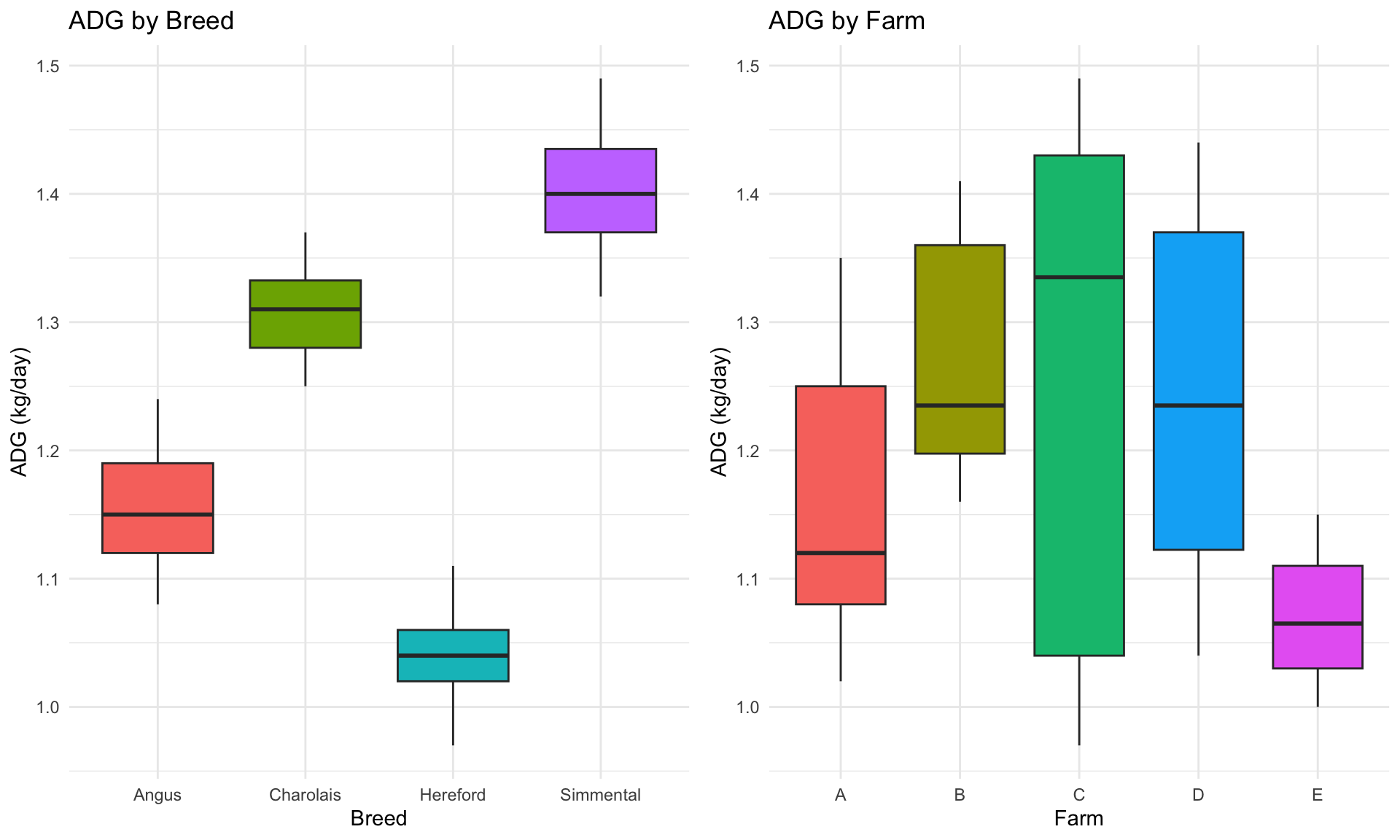
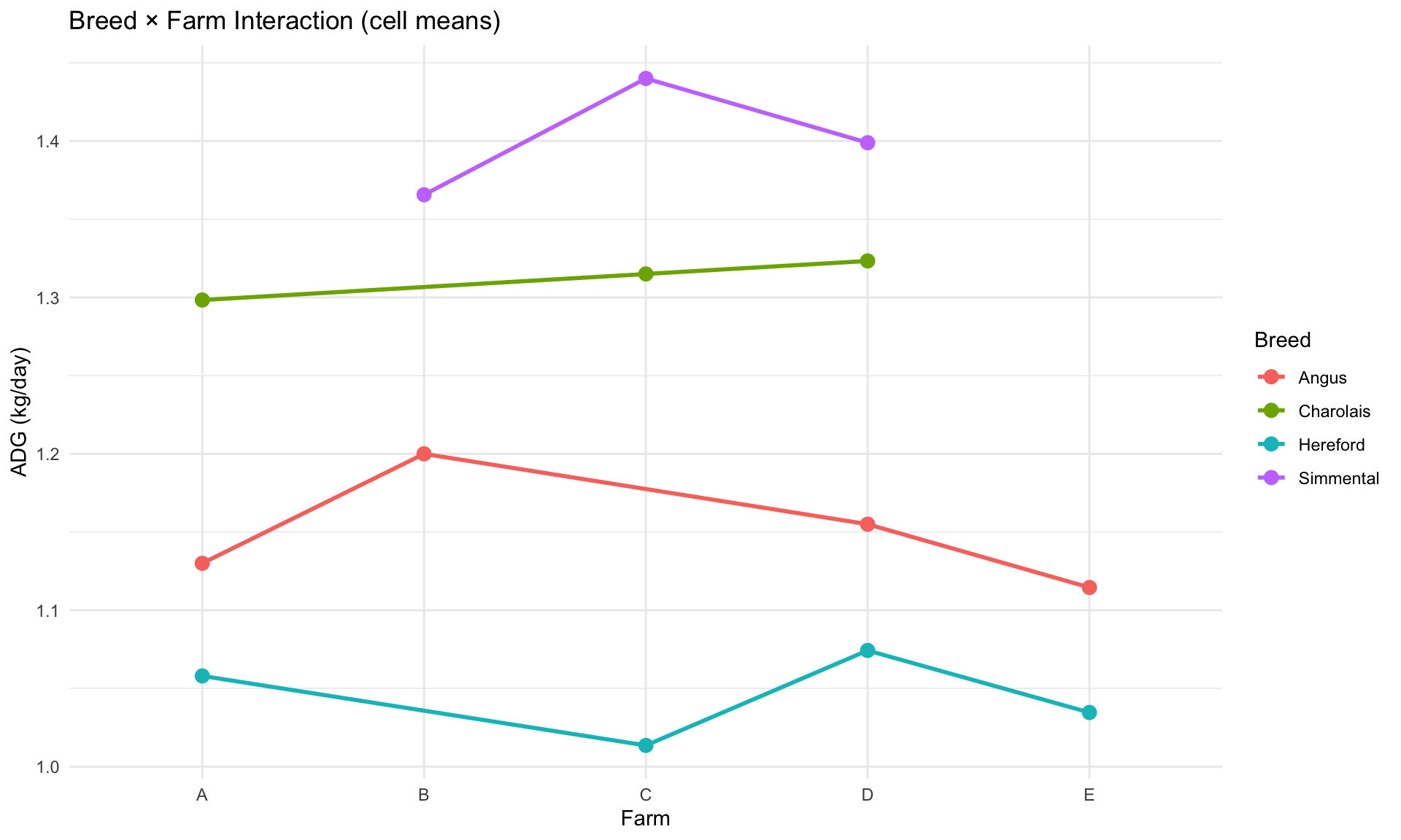
**Observations**:
- Continental breeds (Charolais, Simmental) have higher ADG than British breeds (Angus, Hereford)
- Farm effects evident (B and C higher than E)
- Lines cross → interaction possible (but confounded with missing cells)
---
### Model 1: Breed Only (Cell Means)
```{r}
#| label: beef-model1-breed
# Fit breed-only model (cell means)
fit_breed <- lm(adg ~ breed - 1, data = beef)

cat("Model 1: ADG ~ Breed (cell means)\n")
summary(fit_breed)
# Breed means
breed_means <- coef(fit_breed)
cat("\nBreed means (kg/day):\n")
print(breed_means)
# ANOVA
cat("\nANOVA table:\n")
anova(fit_breed)
# Interpretation
cat("\nInterpretation:\n")
cat("- Charolais highest ADG:", breed_means["breedCharolais"], "kg/day\n")
cat("- Hereford lowest ADG:", breed_means["breedHereford"], "kg/day\n")
cat("- Difference:", breed_means["breedCharolais"] - breed_means["breedHereford"], "kg/day\n")
cat("\nBUT: This ignores farm effects! Breeds not equally distributed across farms.\n")
```
**Problem**: Breed effects are confounded with farm effects because breeds aren't equally represented on all farms.
---
### Model 2: Additive (Breed + Farm)
```{r}
#| label: beef-model2-additive
# Fit additive model
fit_additive <- lm(adg ~ breed + farm, data = beef)

cat("Model 2: ADG ~ Breed + Farm (additive)\n")
summary(fit_additive)
# Type I SS (sequential)
cat("\nType I SS (sequential):\n")
anova(fit_additive)
# Type III SS (each adjusted for others)
library(car)
cat("\nType III SS (each adjusted for others):\n")
Anova(fit_additive, type = 3)
cat("\n→ Note: Type I and Type III give different results!\n")
cat(" With unbalanced data, order matters for Type I.\n")
cat(" Type III tests each effect adjusted for the other.\n")
```
::: {.callout-note}
### Type I vs Type III SS
With unbalanced data, Type I and Type III SS differ:
**Type I (Sequential)**:
- SS(Breed | Intercept), then SS(Farm | Breed)
- Order matters! SS(A|B) ≠ SS(B|A)
- Depends on order effects entered in model
**Type III (Marginal)**:
- SS(Breed | Farm) and SS(Farm | Breed)
- Each effect adjusted for all others
- Order-independent
- **Preferred for unbalanced designs**
**Recommendation**: Use **Type III** for testing with unbalanced data. It asks: "Does breed matter after accounting for farm?" and vice versa.
:::
---
### Model 3: Interaction (Missing Cells)
```{r}
#| label: beef-model3-interaction
# Fit interaction model
fit_interaction <- lm(adg ~ breed * farm, data = beef)

cat("Model 3: ADG ~ Breed * Farm (interaction)\n")
summary(fit_interaction)
# Check which coefficients are NA (non-estimable)
coefs <- coef(fit_interaction)
na_coefs <- names(coefs)[is.na(coefs)]

cat("\nNon-estimable parameters (NA):\n")
print(na_coefs)
cat("\n→ These breed × farm combinations have no data (missing cells)\n")
# Type III ANOVA (may fail with aliased coefficients)
cat("\nAttempting Type III ANOVA:\n")
tryCatch({
  Anova(fit_interaction, type = 3)
}, error = function(e) {
  cat("→ Type III SS cannot be computed due to aliased coefficients\n")
  cat("  This is expected with missing cells in interaction models!\n")
  cat("  Use model comparison with anova() instead.\n")
})
# Test interaction significance
cat("\nTest interaction vs. additive:\n")
anova(fit_additive, fit_interaction)
# Interpretation
if (anova(fit_additive, fit_interaction)$`Pr(>F)`[2] < 0.05) {
  cat("\n→ Interaction is significant (p < 0.05)\n")
  cat("   Breed effects depend on farm!\n")
} else {
  cat("\n→ Interaction not significant (p ≥ 0.05)\n")
  cat("   Additive model sufficient.\n")
}
```
::: {.callout-important}
### Handling Missing Cells
When some breed × farm combinations don't exist:
- Design matrix $\mathbf{X}$ is rank deficient
- R automatically drops redundant parameters (shown as NA)
- Only estimable functions can be tested
- Some comparisons only possible within farms
**Example**: Can't directly compare Angus vs. Simmental on Farm E because Simmental not raised there.
**Solution**: Use marginal means (averaged across farms where both breeds present) via `emmeans`.
:::
---
### Estimable Contrasts with emmeans
```{r}
#| label: beef-estimable-contrasts
#| message: false
library(emmeans)

# Estimated marginal means for breed (averaged across farms)
emm_breed <- emmeans(fit_additive, "breed")

cat("Estimated marginal means (breed):\n")
print(emm_breed)
# Pairwise comparisons
cat("\nPairwise breed comparisons:\n")
pairs_breed <- pairs(emm_breed, adjust = "tukey")
print(pairs_breed)
# Custom contrast: British vs. Continental breeds
# British: Angus, Hereford
# Continental: Charolais, Simmental
contrast_british_continental <- list(
  "British vs Continental" = c(0.5, 0.5, -0.5, -0.5)  # Angus, Char, Here, Simm
)

cat("\nCustom contrast: British vs. Continental breeds:\n")
test_contrast <- contrast(emm_breed, contrast_british_continental)
print(test_contrast)
# Effect size
effect_size <- summary(test_contrast)$estimate
cat("\nEffect size:", effect_size, "kg/day\n")
cat("Continental breeds gain", abs(effect_size), "kg/day more than British breeds (on average).\n")
```
::: {.callout-tip}
### Using emmeans for Unbalanced Data
The `emmeans` package is invaluable for unbalanced designs:
**What it does**:
- Computes **estimated marginal means** (EMMs): breed means averaged across farms, weighted appropriately
- Handles **missing cells** gracefully
- Provides **correct SEs** accounting for unbalanced sample sizes
- Enables **estimable contrasts** only
**When to use**:
- Any unbalanced multi-factor design
- Missing cells
- Want "adjusted means" (breed means accounting for farm differences)
**How to use**:
```r
fit <- lm(response ~ factor1 + factor2, data = data)
emm <- emmeans(fit, "factor1")         # Marginal means
pairs(emm)                              # Pairwise comparisons
contrast(emm, list("Custom" = c(...))) # Custom contrasts
```
:::
---
### Precision Under Unbalanced Data
```{r}
#| label: beef-precision
# Standard errors vary with sample size
emm_summary <- summary(emm_breed)

cat("Standard errors by breed:\n")
print(emm_summary[, c("breed", "emmean", "SE")])
# Relative precision (1/SE²)
emm_summary$rel_precision <- 1 / emm_summary$SE^2

cat("\nRelative precision (1/SE²):\n")
print(emm_summary[, c("breed", "rel_precision")])
# Sample sizes by breed
n_breed <- table(beef$breed)
cat("\nSample sizes:\n")
print(n_breed)
cat("\n→ Breeds with more observations have smaller SEs (more precise).\n")
```
**Key insight**: With unbalanced data, precision differs across groups.
**Formula** (approximately, for simple contrasts):
$$
SE(\hat{\mu}_i - \hat{\mu}_j) \approx \hat{\sigma} \sqrt{\frac{1}{n_i} + \frac{1}{n_j}}
$$
**Implications**:
- Comparisons involving small groups less precise
- Must report sample sizes with means
- Consider weighting in meta-analysis
---
## Practical Guidelines
### Statistical Recommendations
When analyzing unbalanced livestock data, follow these best practices:
**1. Use Type III SS for hypothesis testing**
- Tests each effect adjusted for all others
- Order-independent
- Appropriate for unbalanced designs
**2. Focus on estimable functions**
- Don't interpret non-estimable parameters (NA in R output)
- Use `emmeans` for marginal means
- Test contrasts, not individual parameters
**3. Report sample sizes clearly**
- Always show $n$ by group
- Acknowledge precision differences
- Larger groups have narrower confidence intervals
**4. Use appropriate standard errors**
- `emmeans` computes correct SEs for unbalanced data
- Don't assume equal precision across groups
- $SE(\hat{\mu}_i) \propto 1/\sqrt{n_i}$
**5. Consider model selection carefully**
- Is interaction needed? Test it.
- Are covariates confounded with treatments?
- Document missing cells and their impact
::: {.callout-warning}
### Common Pitfalls with Unbalanced Data
1. **Using Type I SS when order matters**: Type I depends on order effects entered—misleading for unbalanced data
2. **Ignoring confounding**: If groups differ systematically (e.g., all high-performing animals in one group), can't separate cause from selection
3. **Equal weighting when precision differs**: Averaging group means gives equal weight, but some based on $n=5$, others on $n=50$
4. **Interpreting non-estimable parameters**: If R shows NA, that parameter is not estimable—don't try to interpret
5. **Assuming orthogonality**: Unbalanced designs lose orthogonality—effects are correlated
**Always check**:
- Design matrix rank
- Which parameters estimable
- Standard errors vary with $n$
- Type III SS for testing
:::
---
### Experimental Design Implications
**Why balanced designs are preferred**:
1. **Equal precision**: All group means estimated with same accuracy
2. **Orthogonal contrasts**: Effects independent, easier to interpret
3. **Type I = II = III**: All SS types agree
4. **Simpler analysis**: No estimability issues
5. **More power**: For same total $n$, balanced design most powerful
**When unbalanced is unavoidable** (commercial data, missing data, etc.):
1. **Document why**: Animal loss? Selection? Practical constraints?
2. **Analyze appropriately**: Type III SS, `emmeans`, estimable contrasts
3. **Report limitations**: Missing cells, confounding, precision differences
4. **Be transparent**: Show sample sizes, acknowledge bias potential
**For planned experiments**:
- **Aim for balance** when possible
- If unbalanced necessary, plan analysis in advance
- Consider blocking to reduce confounding
---
## Summary
### Conceptual Summary
Real livestock data is messy, but the linear models framework still works—we just need additional tools.
**Key insights from Week 12**:
1. **Cell means model is always full rank**, even with unbalanced data. It directly estimates group means, avoiding singularity issues.
2. **Effects model may be rank deficient** with unbalanced data. Individual $\mu$ and $\alpha_i$ parameters are not uniquely estimable, but contrasts $\alpha_i - \alpha_j$ are.
3. **Generalized inverses solve singular systems**. Any $(\mathbf{X}'\mathbf{X})^-$ works—different g-inverses give different $\mathbf{b}$, but estimable functions $\mathbf{c}'\mathbf{b}$ are always the same.
4. **Estimability is key**: A function $\mathbf{c}'\boldsymbol{\beta}$ is estimable iff $\mathbf{c}' = \mathbf{a}'\mathbf{X}$ for some $\mathbf{a}$. Only estimable functions should be interpreted.
5. **Constraints remove redundancy**: Set-to-zero, sum-to-zero, or weighted constraints make parameters unique, but choice is interpretational—estimable contrasts remain the same.
**For animal breeding applications**:
- We care about **differences** between breeds, sires, or treatments—not absolute values
- Rank deficiency is not a problem for contrasts
- Unbalanced data is the norm in genetic evaluation
- Focus on estimable functions and use appropriate methods (`emmeans`, Type III SS)
::: {.callout-note}
### Looking Ahead
**Week 13: Special Topics I**
- More on constraint systems and different parameterizations
- Types of generalized inverses (Moore-Penrose, reflexive, others)
- Weighted least squares for heterogeneous variances
- Strategic approaches to unbalanced data
**Week 14: Special Topics II**
- Polynomial regression (growth curves, lactation curves)
- Regression through the origin
- **Preview of mixed models**: Adding random effects
- **Henderson's mixed model equations (MME)**: The foundation of BLUP
$$
\begin{bmatrix}
\mathbf{X}'\mathbf{R}^{-1}\mathbf{X} & \mathbf{X}'\mathbf{R}^{-1}\mathbf{Z} \\
\mathbf{Z}'\mathbf{R}^{-1}\mathbf{X} & \mathbf{Z}'\mathbf{R}^{-1}\mathbf{Z} + \mathbf{G}^{-1}
\end{bmatrix}
\begin{bmatrix}
\hat{\boldsymbol{\beta}} \\
\hat{\mathbf{u}}
\end{bmatrix}
=
\begin{bmatrix}
\mathbf{X}'\mathbf{R}^{-1}\mathbf{y} \\
\mathbf{Z}'\mathbf{R}^{-1}\mathbf{y}
\end{bmatrix}
$$
These are augmented normal equations—same tools (generalized inverses, estimability) apply!
Week 12 provides the foundation for understanding mixed models in genetic evaluation.
:::
---
### Key Equations Summary
**Rank-deficient normal equations**:
$$\mathbf{X}'\mathbf{X}\mathbf{b} = \mathbf{X}'\mathbf{y}, \quad r(\mathbf{X}'\mathbf{X}) < p$$
**G-inverse solution**:
$$\mathbf{b} = (\mathbf{X}'\mathbf{X})^-\mathbf{X}'\mathbf{y}$$
**Estimability criterion**:
$$\mathbf{c}'\boldsymbol{\beta} \text{ estimable} \iff \mathbf{c}' = \mathbf{a}'\mathbf{X} \text{ for some } \mathbf{a}$$
**Variance of estimable function**:
$$\text{Var}(\mathbf{c}'\mathbf{b}) = \mathbf{c}'(\mathbf{X}'\mathbf{X})^-\mathbf{c}\sigma^2$$
**t-test for contrast**:
$$t = \frac{\mathbf{c}'\mathbf{b}}{\sqrt{\mathbf{c}'(\mathbf{X}'\mathbf{X})^-\mathbf{c}\hat{\sigma}^2}} \sim t(n - r(\mathbf{X}))$$
**SE for unbalanced contrast** (approximate):
$$SE(\hat{\mu}_i - \hat{\mu}_j) \approx \hat{\sigma}\sqrt{\frac{1}{n_i} + \frac{1}{n_j}}$$
---
### Cross-References
- **Previous**: [Week 11: Model Diagnostics](../Week11_Diagnostics/Week11_Diagnostics.qmd)
- **Next**: [Week 13: Special Topics I](../Week13_SpecialTopicsI/Week13_SpecialTopicsI.qmd)
---
### References
::: {.callout-tip}
### Additional Resources
**Textbooks**:
- Searle, S. R. (1971). *Linear Models*. Wiley. [Classic reference on rank deficiency and estimability]
- Milliken, G. A., & Johnson, D. E. (2009). *Analysis of Messy Data, Volume 1: Designed Experiments* (2nd ed.). CRC Press.
- Henderson, C. R. (1984). *Applications of Linear Models in Animal Breeding*. University of Guelph.
**R Packages**:
- `MASS::ginv()`: Moore-Penrose inverse
- `emmeans`: Estimated marginal means and contrasts
- `car::Anova()`: Type II and Type III SS
**Vignettes**:
- `emmeans` vignette on estimability: `vignette("basics", package="emmeans")`
- FAQs on unbalanced ANOVA: `vignette("FAQs", package="emmeans")`
**Papers**:
- Searle, S. R., Speed, F. M., & Milliken, G. A. (1980). Population marginal means in the linear model: An alternative to least squares means. *The American Statistician*, 34(4), 216-221.
:::