---
title: "Week 4: Simple Linear Regression"
format:
html:
toc: true
toc-depth: 3
number-sections: true
code-fold: false
code-tools: true
---
::: {.callout-note icon=false}
## Learning Objectives
By the end of this week, you will be able to:
1. **Derive** **least squares estimates** for **simple linear regression** from first principles
2. **Interpret** **slope** and **intercept parameters** in biological context
3. **Make predictions** and compute **residuals** for new observations
4. **Understand** the geometry of **least squares** and the concept of **"best fit"**
:::
## Why Simple Linear Regression Matters
Simple linear regression is one of the most fundamental and widely used statistical methods in animal breeding and genetics. It allows us to quantify relationships between two continuous variables and make predictions.
**Common applications in livestock science:**
- **Growth curves**: Predicting animal weight from age (broilers, pigs, beef cattle)
- **Feed efficiency**: Relating feed intake to weight gain
- **Lactation curves**: Modeling milk yield over days in milk (dairy cattle)
- **Carcass traits**: Predicting carcass weight from live weight
- **Economic traits**: Relating input costs to productivity measures
::: {.callout-note}
## Connection to Previous Weeks
In [Week 3](#sec-week03), we learned how to build design matrices for different types of predictors. Simple linear regression uses a design matrix with just two columns: one for the intercept (all 1s) and one for our predictor variable. This week, we'll learn how to estimate the parameters in this model and interpret the results.
:::
::: {.callout-tip}
## Why Learn Regression from First Principles?
Understanding how to derive regression estimates manually gives you:
- Deep insight into what statistical software is actually doing
- Ability to build custom solvers for specialized problems
- Foundation for understanding more complex models (multiple regression, ANOVA, mixed models)
- Confidence to troubleshoot when results seem unexpected
:::
## The Simple Linear Regression Model
### Model Specification
In simple linear regression, we model the relationship between a **response variable** $y$ and a **predictor variable** $x$ using a straight line:
$$
y_i = \beta_0 + \beta_1 x_i + e_i, \quad i = 1, 2, \ldots, n
$$ {#eq-simple-regression}
where:
- $y_i$ = observed response for observation $i$ (scalar)
- $x_i$ = predictor value for observation $i$ (scalar)
- $\beta_0$ = **intercept** parameter (scalar, unknown)
- $\beta_1$ = **slope** parameter (scalar, unknown)
- $e_i$ = random error for observation $i$ (scalar, unobserved)
- $n$ = total number of observations (scalar)
**Interpretation:**
- $\beta_0$ represents the expected value of $y$ when $x = 0$
- $\beta_1$ represents the expected change in $y$ for a one-unit increase in $x$
- $e_i$ captures all variation in $y$ not explained by $x$
### Matrix Form
We can write the simple linear regression model in matrix form as:
$$
\mathbf{y} = \mathbf{X}\boldsymbol{\beta} + \mathbf{e}
$$ {#eq-matrix-regression}
where:
$$
\mathbf{y} = \begin{bmatrix} y_1 \\ y_2 \\ \vdots \\ y_n \end{bmatrix}_{n \times 1}, \quad
\mathbf{X} = \begin{bmatrix} 1 & x_1 \\ 1 & x_2 \\ \vdots & \vdots \\ 1 & x_n \end{bmatrix}_{n \times 2}, \quad
\boldsymbol{\beta} = \begin{bmatrix} \beta_0 \\ \beta_1 \end{bmatrix}_{2 \times 1}, \quad
\mathbf{e} = \begin{bmatrix} e_1 \\ e_2 \\ \vdots \\ e_n \end{bmatrix}_{n \times 1}
$$
**Key observations:**
- $\mathbf{y}$ is an $n \times 1$ vector of responses
- $\mathbf{X}$ is an $n \times 2$ **design matrix** (first column is all 1s for intercept, second column contains the $x$ values)
- $\boldsymbol{\beta}$ is a $2 \times 1$ vector of unknown parameters
- $\mathbf{e}$ is an $n \times 1$ vector of errors
::: {.callout-note}
## Design Matrix Structure
The first column of $\mathbf{X}$ (all 1s) corresponds to the intercept $\beta_0$. The second column contains the predictor values and corresponds to the slope $\beta_1$. This structure comes directly from our Week 3 discussion of building design matrices for continuous predictors.
:::
### Model Assumptions
For valid inference, we make the following assumptions about the errors:
::: {.callout-important}
## Gauss-Markov Assumptions
1. **Linearity**: The relationship between $x$ and $y$ is linear
2. **Zero mean**: $E(\mathbf{e}) = \mathbf{0}$ (errors have expected value of zero)
3. **Homoscedasticity**: $\text{Var}(e_i) = \sigma^2$ for all $i$ (constant variance)
4. **Independence**: $\text{Cov}(e_i, e_j) = 0$ for all $i \neq j$ (errors are uncorrelated)
These can be summarized as: $\text{Var}(\mathbf{e}) = \sigma^2 \mathbf{I}_n$
For hypothesis testing, we often add a fifth assumption:
5. **Normality**: $\mathbf{e} \sim N(\mathbf{0}, \sigma^2 \mathbf{I}_n)$ (errors are normally distributed)
:::
Under these assumptions, the least squares estimates we derive will have optimal properties (which we'll prove in Week 5).
## Deriving the Normal Equations
Our goal is to find estimates $b_0$ and $b_1$ for the unknown parameters $\beta_0$ and $\beta_1$. We'll use the **method of least squares**, which minimizes the sum of squared residuals.
### The Least Squares Criterion
We want to find values of $\beta_0$ and $\beta_1$ that minimize:
$$
S(\beta_0, \beta_1) = \sum_{i=1}^{n} (y_i - \beta_0 - \beta_1 x_i)^2
$$
In matrix notation, this is:
$$
S(\boldsymbol{\beta}) = (\mathbf{y} - \mathbf{X}\boldsymbol{\beta})'(\mathbf{y} - \mathbf{X}\boldsymbol{\beta}) = \|\mathbf{y} - \mathbf{X}\boldsymbol{\beta}\|^2
$$
### Constructing the Normal Equations
To minimize $S(\boldsymbol{\beta})$, we'll use matrix algebra. First, let's compute $\mathbf{X}'\mathbf{X}$ and $\mathbf{X}'\mathbf{y}$.
**Computing $\mathbf{X}'\mathbf{X}$:**
$$
\mathbf{X}' = \begin{bmatrix} 1 & 1 & \cdots & 1 \\ x_1 & x_2 & \cdots & x_n \end{bmatrix}_{2 \times n}
$$
$$
\mathbf{X}'\mathbf{X} = \begin{bmatrix} 1 & 1 & \cdots & 1 \\ x_1 & x_2 & \cdots & x_n \end{bmatrix} \begin{bmatrix} 1 & x_1 \\ 1 & x_2 \\ \vdots & \vdots \\ 1 & x_n \end{bmatrix}
$$
$$
\mathbf{X}'\mathbf{X} = \begin{bmatrix} n & \sum_{i=1}^{n} x_i \\ \sum_{i=1}^{n} x_i & \sum_{i=1}^{n} x_i^2 \end{bmatrix}_{2 \times 2}
$$ {#eq-xtx}
**Computing $\mathbf{X}'\mathbf{y}$:**
$$
\mathbf{X}'\mathbf{y} = \begin{bmatrix} 1 & 1 & \cdots & 1 \\ x_1 & x_2 & \cdots & x_n \end{bmatrix} \begin{bmatrix} y_1 \\ y_2 \\ \vdots \\ y_n \end{bmatrix}
$$
$$
\mathbf{X}'\mathbf{y} = \begin{bmatrix} \sum_{i=1}^{n} y_i \\ \sum_{i=1}^{n} x_i y_i \end{bmatrix}_{2 \times 1}
$$ {#eq-xty}
The **normal equations** are:
$$
\mathbf{X}'\mathbf{X}\mathbf{b} = \mathbf{X}'\mathbf{y}
$$ {#eq-normal-equations}
Substituting our results:
$$
\begin{bmatrix} n & \sum x_i \\ \sum x_i & \sum x_i^2 \end{bmatrix} \begin{bmatrix} b_0 \\ b_1 \end{bmatrix} = \begin{bmatrix} \sum y_i \\ \sum x_i y_i \end{bmatrix}
$$ {#eq-normal-expanded}
### Solving the Normal Equations
The matrix solution is:
$$
\mathbf{b} = (\mathbf{X}'\mathbf{X})^{-1}\mathbf{X}'\mathbf{y}
$$ {#eq-matrix-solution}
For a $2 \times 2$ matrix $\mathbf{A} = \begin{bmatrix} a & b \\ c & d \end{bmatrix}$, the inverse is:
$$
\mathbf{A}^{-1} = \frac{1}{ad - bc} \begin{bmatrix} d & -b \\ -c & a \end{bmatrix}
$$
For $\mathbf{X}'\mathbf{X}$:
- $a = n$, $b = \sum x_i$, $c = \sum x_i$, $d = \sum x_i^2$
- Determinant: $|\mathbf{X}'\mathbf{X}| = n\sum x_i^2 - (\sum x_i)^2$
$$
(\mathbf{X}'\mathbf{X})^{-1} = \frac{1}{n\sum x_i^2 - (\sum x_i)^2} \begin{bmatrix} \sum x_i^2 & -\sum x_i \\ -\sum x_i & n \end{bmatrix}
$$ {#eq-xtx-inverse}
### Closed-Form Solutions
We can also derive algebraic formulas. From @eq-normal-expanded:
**Equation 1:** $n b_0 + b_1 \sum x_i = \sum y_i$
**Equation 2:** $b_0 \sum x_i + b_1 \sum x_i^2 = \sum x_i y_i$
From Equation 1: $b_0 = \bar{y} - b_1 \bar{x}$ where $\bar{x} = \frac{1}{n}\sum x_i$ and $\bar{y} = \frac{1}{n}\sum y_i$
Substituting into Equation 2 and simplifying:
$$
b_1 = \frac{\sum_{i=1}^{n}(x_i - \bar{x})(y_i - \bar{y})}{\sum_{i=1}^{n}(x_i - \bar{x})^2} = \frac{\sum x_i y_i - n\bar{x}\bar{y}}{\sum x_i^2 - n\bar{x}^2}
$$ {#eq-slope}
$$
b_0 = \bar{y} - b_1 \bar{x}
$$ {#eq-intercept}
::: {.callout-tip}
## Two Equivalent Approaches
The **matrix approach** $\mathbf{b} = (\mathbf{X}'\mathbf{X})^{-1}\mathbf{X}'\mathbf{y}$ is general and extends to multiple regression.
The **closed-form** formulas for $b_0$ and $b_1$ are computationally simpler for simple regression and provide intuition: $b_1$ is the ratio of covariation to variation in $x$.
Both give identical results!
:::
## Small Numerical Example: Broiler Growth
Let's work through a complete example by hand. We'll use data on broiler chicken weight (kg) versus age (days).
### The Data
| Observation | Age (days), $x_i$ | Weight (kg), $y_i$ |
|-------------|-------------------|--------------------|
| 1 | 21 | 0.50 |
| 2 | 28 | 0.90 |
| 3 | 35 | 1.40 |
| 4 | 42 | 1.90 |
**Sample size:** $n = 4$
### Step 1: Calculate Summary Statistics
$$
\sum x_i = 21 + 28 + 35 + 42 = 126
$$
$$
\sum y_i = 0.50 + 0.90 + 1.40 + 1.90 = 4.70
$$
$$
\bar{x} = \frac{126}{4} = 31.5 \text{ days}
$$
$$
\bar{y} = \frac{4.70}{4} = 1.175 \text{ kg}
$$
$$
\sum x_i^2 = 21^2 + 28^2 + 35^2 + 42^2 = 441 + 784 + 1225 + 1764 = 4214
$$
$$
\sum x_i y_i = (21)(0.50) + (28)(0.90) + (35)(1.40) + (42)(1.90)
$$
$$
= 10.5 + 25.2 + 49.0 + 79.8 = 164.5
$$
### Step 2: Construct $\mathbf{X}'\mathbf{X}$
Using @eq-xtx:
$$
\mathbf{X}'\mathbf{X} = \begin{bmatrix} 4 & 126 \\ 126 & 4214 \end{bmatrix}
$$
### Step 3: Construct $\mathbf{X}'\mathbf{y}$
Using @eq-xty:
$$
\mathbf{X}'\mathbf{y} = \begin{bmatrix} 4.70 \\ 164.5 \end{bmatrix}
$$
### Step 4: Compute $(\mathbf{X}'\mathbf{X})^{-1}$
Determinant: $|\mathbf{X}'\mathbf{X}| = (4)(4214) - (126)(126) = 16856 - 15876 = 980$
Using @eq-xtx-inverse:
$$
(\mathbf{X}'\mathbf{X})^{-1} = \frac{1}{980} \begin{bmatrix} 4214 & -126 \\ -126 & 4 \end{bmatrix} = \begin{bmatrix} 4.3 & -0.1286 \\ -0.1286 & 0.0041 \end{bmatrix}
$$
(Values rounded to 4 decimal places)
### Step 5: Compute $\mathbf{b} = (\mathbf{X}'\mathbf{X})^{-1}\mathbf{X}'\mathbf{y}$
$$
\mathbf{b} = \begin{bmatrix} 4.3 & -0.1286 \\ -0.1286 & 0.0041 \end{bmatrix} \begin{bmatrix} 4.70 \\ 164.5 \end{bmatrix}
$$
$$
b_0 = (4.3)(4.70) + (-0.1286)(164.5) = 20.21 - 21.15 = -0.94
$$
$$
b_1 = (-0.1286)(4.70) + (0.0041)(164.5) = -0.604 + 0.674 = 0.0667
$$
Therefore:
$$
\mathbf{b} = \begin{bmatrix} b_0 \\ b_1 \end{bmatrix} = \begin{bmatrix} -0.94 \\ 0.0667 \end{bmatrix}
$$
### Step 6: Verify with Closed-Form Formulas
Using @eq-slope:
$$
b_1 = \frac{\sum x_i y_i - n\bar{x}\bar{y}}{\sum x_i^2 - n\bar{x}^2} = \frac{164.5 - (4)(31.5)(1.175)}{4214 - (4)(31.5)^2}
$$
$$
= \frac{164.5 - 148.05}{4214 - 3969} = \frac{16.45}{245} = 0.0667 \text{ kg/day}
$$
Using @eq-intercept:
$$
b_0 = \bar{y} - b_1\bar{x} = 1.175 - (0.0667)(31.5) = 1.175 - 2.101 = -0.926 \text{ kg}
$$
(Slight differences due to rounding)
### Step 7: Write the Fitted Regression Equation
$$
\hat{y}_i = b_0 + b_1 x_i = -0.94 + 0.0667 x_i
$$
### Step 8: Calculate Fitted Values
For each observation, $\hat{y}_i = -0.94 + 0.0667 x_i$:
| $i$ | $x_i$ | $y_i$ | $\hat{y}_i$ |
|-----|-------|-------|-------------|
| 1 | 21 | 0.50 | 0.46 |
| 2 | 28 | 0.90 | 0.93 |
| 3 | 35 | 1.40 | 1.39 |
| 4 | 42 | 1.90 | 1.86 |
### Step 9: Calculate Residuals
Residuals: $e_i = y_i - \hat{y}_i$
| $i$ | $y_i$ | $\hat{y}_i$ | $e_i$ |
|-----|-------|-------------|-------|
| 1 | 0.50 | 0.46 | 0.04 |
| 2 | 0.90 | 0.93 | -0.03 |
| 3 | 1.40 | 1.39 | 0.01 |
| 4 | 1.90 | 1.86 | 0.04 |
**Check:** $\sum e_i = 0.04 - 0.03 + 0.01 + 0.04 = 0.06 \approx 0$ ✓ (small rounding error)
### Step 10: Calculate SSE
$$
\text{SSE} = \sum_{i=1}^{n} e_i^2 = (0.04)^2 + (-0.03)^2 + (0.01)^2 + (0.04)^2
$$
$$
= 0.0016 + 0.0009 + 0.0001 + 0.0016 = 0.0042 \text{ kg}^2
$$
### Biological Interpretation
::: {.callout-note}
## What Do These Estimates Mean?
**Slope ($b_1 = 0.0667$ kg/day):**
- For every additional day of age, broiler weight increases by approximately 0.067 kg (or 67 grams per day)
- This is the **growth rate** of the broilers during this period
- This is within the typical range for modern broiler chickens
**Intercept ($b_0 = -0.94$ kg):**
- Mathematically, this is the predicted weight when age = 0 days
- Biologically, this doesn't make sense (negative weight!)
- This is because we're **extrapolating** far beyond our data (ages 21-42 days)
- The intercept is still useful for making the line fit well within our data range
:::
### Making Predictions
**Predict weight at age 30 days:**
$$
\hat{y} = -0.94 + 0.0667(30) = -0.94 + 2.00 = 1.06 \text{ kg}
$$
This is an **interpolation** (within the range of observed ages), so it's reliable.
::: {.callout-warning}
## Extrapolation vs. Interpolation
**Interpolation**: Predicting within the range of observed $x$ values (21-42 days in our example). Generally reliable.
**Extrapolation**: Predicting outside the range of observed $x$ values (e.g., age = 60 days or age = 7 days). Can be unreliable because the linear relationship may not hold outside the observed range.
Always be cautious about extrapolation!
:::
### R Implementation
Let's verify our hand calculations using R:
```{r}
#| label: broiler-manual-calculation
#| message: false
# Enter the data
age <- c(21, 28, 35, 42)           # Age in days (predictor)
weight <- c(0.50, 0.90, 1.40, 1.90)  # Weight in kg (response)
n <- length(age)                   # Sample size

# Create design matrix X
X <- cbind(1, age)  # First column: intercept (all 1s), Second column: age
print("Design matrix X:")
print(X)
# Compute X'X (2x2 matrix)
XtX <- t(X) %*% X
print("X'X:")
print(XtX)
# Compute X'y (2x1 vector)
Xty <- t(X) %*% weight
print("X'y:")
print(Xty)
# Compute (X'X)^(-1)
XtX_inv <- solve(XtX)
print("(X'X)^(-1):")
print(XtX_inv)
# Compute b = (X'X)^(-1) X'y
b <- XtX_inv %*% Xty
print("Coefficient estimates b:")
print(b)
# Extract individual coefficients
b0 <- b[1, 1]  # Intercept
b1 <- b[2, 1]  # Slope
cat("\nIntercept (b0):", round(b0, 4), "kg\n")
cat("Slope (b1):", round(b1, 4), "kg/day\n")
# Calculate fitted values
y_hat <- X %*% b
print("Fitted values:")
print(y_hat)
# Calculate residuals
residuals <- weight - y_hat
print("Residuals:")
print(residuals)
# Check that residuals sum to (approximately) zero
cat("\nSum of residuals:", sum(residuals), "\n")
# Calculate SSE (Sum of Squared Errors)
SSE <- sum(residuals^2)
cat("SSE:", SSE, "kg^2\n")
# Verify with lm()
fit_lm <- lm(weight ~ age)
cat("\n--- Verification with lm() ---\n")
print(summary(fit_lm)$coefficients)
cat("\nOur b0:", b0, "vs lm() intercept:", coef(fit_lm)[1], "\n")
cat("Our b1:", b1, "vs lm() slope:", coef(fit_lm)[2], "\n")
```
Perfect! Our manual calculations match R's `lm()` function.
## Understanding Fitted Values and Residuals
### Fitted Values
**Fitted values** (or **predicted values**) $\hat{y}_i$ are the values predicted by our regression model:
$$
\hat{y}_i = b_0 + b_1 x_i
$$
In matrix form:
$$
\hat{\mathbf{y}} = \mathbf{X}\mathbf{b}
$$
These represent the points on the regression line. For each observed $x_i$, we have a corresponding predicted value $\hat{y}_i$.
### Residuals
**Residuals** $e_i$ are the differences between observed and fitted values:
$$
e_i = y_i - \hat{y}_i
$$
In matrix form:
$$
\mathbf{e} = \mathbf{y} - \hat{\mathbf{y}} = \mathbf{y} - \mathbf{X}\mathbf{b}
$$
Residuals represent the **unexplained variation** in $y$ after accounting for $x$.
### Properties of Least Squares Residuals
For a regression model with an intercept, the residuals have important properties:
::: {.callout-important}
## Key Properties
1. **Residuals sum to zero:** $\sum_{i=1}^{n} e_i = 0$
2. **Residuals are orthogonal to predictors:** $\sum_{i=1}^{n} x_i e_i = 0$
3. **Residuals are orthogonal to fitted values:** $\sum_{i=1}^{n} \hat{y}_i e_i = 0$
These properties come directly from the normal equations $\mathbf{X}'\mathbf{e} = \mathbf{0}$.
:::
::: {.callout-note}
## Preview to Week 5
In Week 5 (Least Squares Theory), we'll prove these properties mathematically and explore the geometric interpretation using projection matrices. For now, it's important to verify these properties hold in our examples.
:::
### Sum of Squared Errors (SSE)
The **sum of squared errors** (also called the **residual sum of squares**) measures the total unexplained variation:
$$
\text{SSE} = \sum_{i=1}^{n} e_i^2 = \mathbf{e}'\mathbf{e}
$$ {#eq-sse}
This is the quantity we minimized to find our least squares estimates. A smaller SSE indicates a better fit.
## The Geometry of Least Squares
### Visualizing the Regression Line
The regression line $\hat{y} = b_0 + b_1 x$ is the "best fitting" line through the data points in the sense that it minimizes the sum of squared vertical distances (residuals).
```{r}
#| label: regression-visualization
#| message: false
#| fig-width: 7
#| fig-height: 5
# Create scatter plot with regression line
plot(age, weight,
     pch = 16, col = "blue", cex = 1.5,
     xlab = "Age (days)",
     ylab = "Weight (kg)",
     main = "Broiler Growth: Simple Linear Regression",
     xlim = c(15, 45), ylim = c(0, 2.5))

# Add regression line
abline(b0, b1, col = "red", lwd = 2)

# Add residual lines (vertical distances from points to line)
for (i in 1:n) {
  segments(age[i], weight[i], age[i], y_hat[i],
           col = "darkgreen", lty = 2, lwd = 1.5)
}

# Add legend
legend("topleft",
       legend = c("Observed data", "Fitted line", "Residuals"),
       col = c("blue", "red", "darkgreen"),
       pch = c(16, NA, NA),
       lty = c(NA, 1, 2),
       lwd = c(NA, 2, 1.5))

# Add equation to plot
equation <- paste0("y = ", round(b0, 2), " + ", round(b1, 3), "x")
text(35, 0.5, equation, cex = 1.2, col = "red")
```
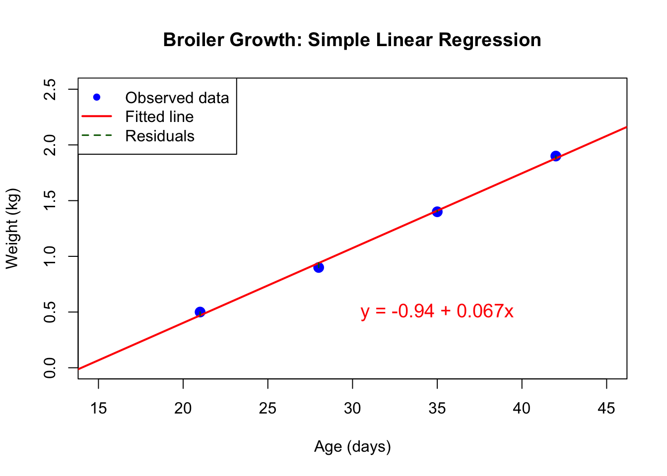
**Interpretation:**
- **Blue points**: Observed data (age, weight)
- **Red line**: Fitted regression line
- **Green dashed lines**: Residuals (vertical distances from points to line)
The least squares method finds the line that makes the sum of the squared lengths of these green lines as small as possible.
### The Least Squares Criterion
We are minimizing:
$$
\text{SSE} = \sum_{i=1}^{n} e_i^2 = \sum_{i=1}^{n} (y_i - b_0 - b_1 x_i)^2
$$
This is equivalent to minimizing the sum of the squared lengths of the residual lines in the plot above.
::: {.callout-note}
## Why Square the Residuals?
We square the residuals for several reasons:
1. **Positive values**: Squaring makes all deviations positive (otherwise positive and negative residuals would cancel)
2. **Penalizes large errors**: Squaring gives more weight to large deviations
3. **Mathematical convenience**: Leads to linear normal equations (easier to solve)
4. **Optimal properties**: Under certain conditions, least squares estimators are BLUE (Best Linear Unbiased Estimators) - we'll prove this in Week 5
:::
## Realistic Application: Dairy Lactation Curves
Now let's apply simple linear regression to a more realistic dataset. We'll analyze milk yield over the first 100 days of lactation for 30 Holstein dairy cows.
### Background: Lactation Curves
Dairy cows produce milk after giving birth (calving). Milk production:
- Rises rapidly in the first few weeks (peak lactation around 60 days)
- Gradually declines throughout lactation
- True lactation curves are **nonlinear** (often modeled with Wood's curve or polynomial functions)
For the **first 100 days** of lactation, a **linear approximation** can sometimes be reasonable as a first-order model, though we'll note its limitations.
::: {.callout-tip}
## Connecting to Advanced Topics
In Week 14, we'll learn about **polynomial regression** to model nonlinear relationships like lactation curves more accurately. For now, we'll use simple linear regression as an introduction to the process.
:::
### Load and Explore the Data
```{r}
#| label: dairy-load-data
#| message: false
# Load the data
dairy <- read.csv("data/dairy_lactation.csv")

# Display first few rows
head(dairy, 10)
# Summary statistics
cat("Number of observations:", nrow(dairy), "\n")
cat("Days in milk range:", range(dairy$days_in_milk), "\n")
cat("Milk yield range:", range(dairy$milk_yield_kg), "\n\n")
# Summary statistics by variable
summary(dairy)
```
### Exploratory Scatter Plot
```{r}
#| label: dairy-scatter
#| message: false
#| fig-width: 8
#| fig-height: 6
# Create scatter plot
plot(dairy$days_in_milk, dairy$milk_yield_kg,
     pch = 16, col = "darkblue", cex = 1.2,
     xlab = "Days in Milk (DIM)",
     ylab = "Milk Yield (kg/day)",
     main = "Dairy Lactation: Milk Yield vs. Days in Milk")

# Add grid for easier reading
grid()
```
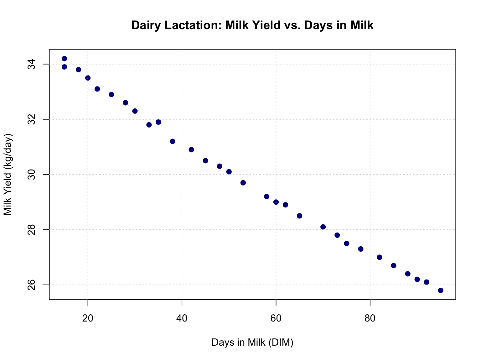
**Observations:**
- There appears to be a **negative linear trend**: milk yield decreases as days in milk increases
- The relationship looks approximately linear for this range (15-95 days)
- Some scatter around the trend, which is expected biological variation
### Build the Model Manually
```{r}
#| label: dairy-manual-model
#| message: false
# Extract variables
x <- dairy$days_in_milk
y <- dairy$milk_yield_kg
n <- length(x)

cat("Sample size n =", n, "\n\n")
# Build design matrix
X <- cbind(1, x)
cat("Design matrix X dimensions:", dim(X), "\n")
cat("First 5 rows of X:\n")
print(head(X, 5))
# Compute X'X
XtX <- t(X) %*% X
cat("\nX'X (2x2 matrix):\n")
print(XtX)
# Compute X'y
Xty <- t(X) %*% y
cat("\nX'y (2x1 vector):\n")
print(Xty)
# Solve normal equations: b = (X'X)^(-1) X'y
b <- solve(XtX) %*% Xty
cat("\nLeast squares estimates:\n")
cat("b0 (intercept):", b[1,1], "kg/day\n")
cat("b1 (slope):", b[2,1], "kg/(day·DIM)\n")
# Calculate fitted values
y_hat <- X %*% b

# Calculate residuals
e <- y - y_hat

# Calculate SSE
SSE <- sum(e^2)
cat("\nSum of Squared Errors (SSE):", round(SSE, 4), "kg^2\n")
# Check properties of residuals
cat("\nResidual properties:\n")
cat("Sum of residuals:", round(sum(e), 10), "(should be ~0)\n")
cat("Sum of x*e:", round(sum(x * e), 10), "(should be ~0)\n")
```
### Compare with lm()
```{r}
#| label: dairy-compare-lm
#| message: false
# Fit using lm()
fit_dairy <- lm(milk_yield_kg ~ days_in_milk, data = dairy)

cat("Comparison: Manual vs lm()\n")
cat("-----------------------------\n")
cat("Intercept:\n")
cat(" Manual:", b[1,1], "\n")
cat(" lm(): ", coef(fit_dairy)[1], "\n")
cat("Slope:\n")
cat(" Manual:", b[2,1], "\n")
cat(" lm(): ", coef(fit_dairy)[2], "\n")
cat("\nDifference (should be near zero):\n")
cat(" Intercept:", b[1,1] - coef(fit_dairy)[1], "\n")
cat(" Slope: ", b[2,1] - coef(fit_dairy)[2], "\n")
# Display lm() summary
cat("\n--- lm() Summary ---\n")
summary(fit_dairy)
```
Perfect agreement! Our manual calculation exactly matches R's `lm()`.
### Visualize the Fitted Model
```{r}
#| label: dairy-fitted-plot
#| message: false
#| fig-width: 8
#| fig-height: 6
# Plot data and fitted line
plot(dairy$days_in_milk, dairy$milk_yield_kg,
     pch = 16, col = "darkblue", cex = 1.2,
     xlab = "Days in Milk (DIM)",
     ylab = "Milk Yield (kg/day)",
     main = "Dairy Lactation: Fitted Regression Line")

# Add fitted line
abline(b[1,1], b[2,1], col = "red", lwd = 2)

# Add equation
equation_text <- paste0("Milk Yield = ", round(b[1,1], 2), " + ",
                       round(b[2,1], 4), " × DIM")
text(70, 34, equation_text, cex = 1.1, col = "red")

# Add legend
legend("topright",
       legend = c("Observed data", "Fitted regression line"),
       col = c("darkblue", "red"),
       pch = c(16, NA),
       lty = c(NA, 1),
       lwd = c(NA, 2))

grid()
```
### Biological Interpretation
::: {.callout-important}
## Interpreting the Dairy Model
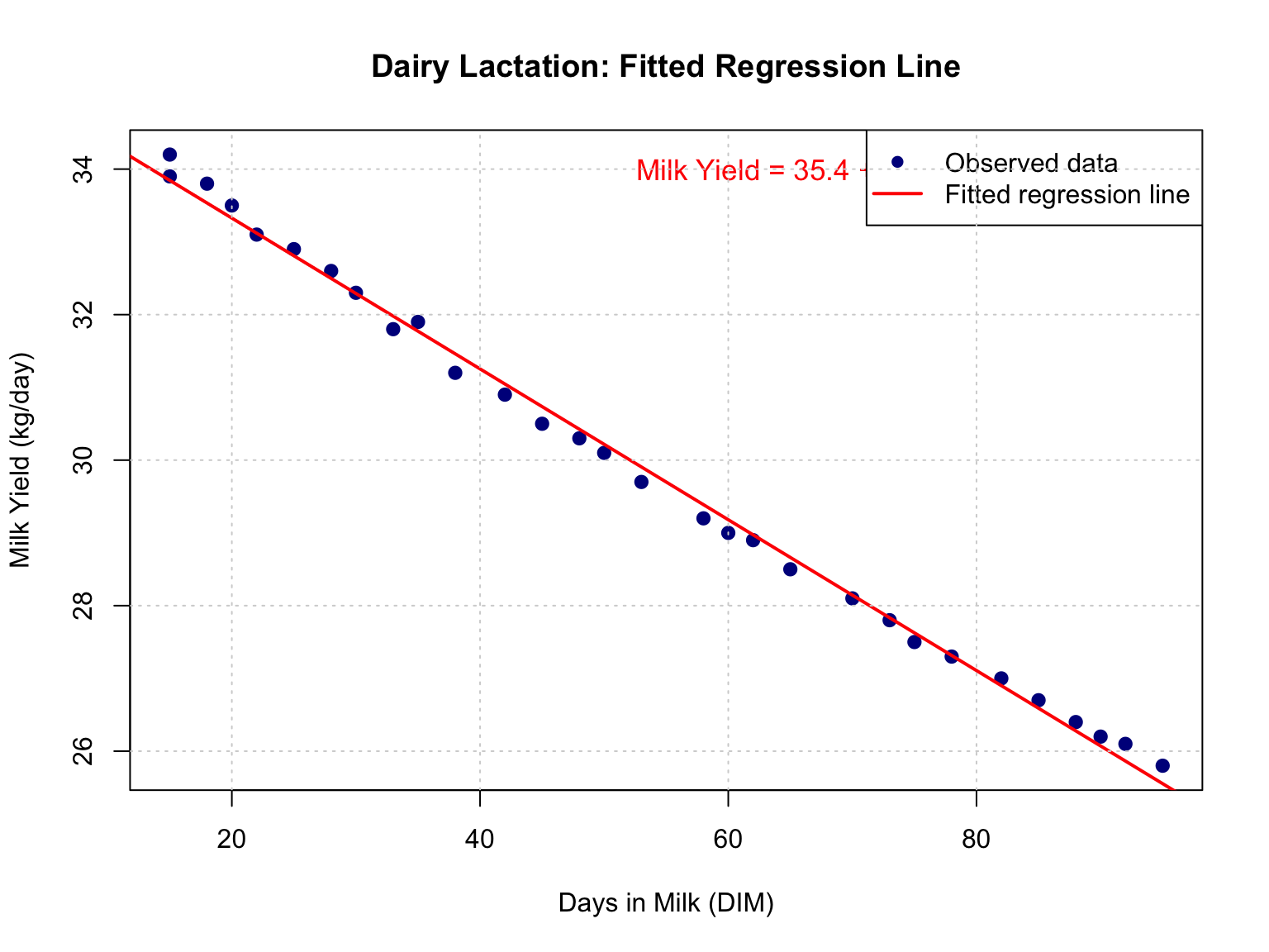
**Intercept ($b_0 \approx 35.15$ kg/day):**
- This is the estimated milk yield at day 0 (calving)
- Biologically, cows don't produce this much milk immediately at calving
- This is a **mathematical extrapolation** beyond our data range (DIM 15-95)
- The true lactation curve is nonlinear near calving
**Slope ($b_1 \approx -0.0874$ kg/day per DIM):**
- For each additional day in milk, yield decreases by approximately 0.087 kg/day
- This is the **rate of decline** in the linear portion of the lactation curve
- Over 10 days, we expect a decline of about 0.87 kg/day
- This rate is consistent with the declining phase of lactation
**Model fit:**
- SSE = 18.58 kg², which represents unexplained variation
- The linear model captures the general declining trend
- However, true lactation curves are curvilinear (peak early, then decline)
- A polynomial model (Week 14) would fit better
:::
### Making Predictions
Let's predict milk yield at different days in milk:
```{r}
#| label: dairy-predictions
#| message: false
# Predictions at specific DIM values
dim_values <- c(20, 40, 60, 80)

cat("Predictions:\n")
cat("-----------------------------\n")
for (dim_val in dim_values) {
  predicted_yield <- b[1,1] + b[2,1] * dim_val
  cat("DIM =", dim_val, "days: Predicted yield =",
      round(predicted_yield, 2), "kg/day\n")
}
```
All these predictions are **interpolations** (within the 15-95 day range), so they are reasonably reliable for this linear approximation.
## Building Your Own Simple Regression Solver
Now that we understand the mathematics, let's build a reusable function that performs simple linear regression from scratch.
```{r}
#| label: custom-solver
#| message: false
#' Simple Linear Regression Solver
#'
#' Fits a simple linear regression model y = b0 + b1*x + e
#' using the least squares method
#'
#' @param x Numeric vector of predictor values
#' @param y Numeric vector of response values
#' @return A list containing regression results
simple_lm <- function(x, y) {

  # Input validation
  if (length(x) != length(y)) {
    stop("x and y must have the same length")
  }
  if (length(x) < 2) {
    stop("Need at least 2 observations")
  }

  # Sample size
  n <- length(x)

  # Construct design matrix X (n x 2)
  X <- cbind(1, x)

  # Compute X'X (2 x 2)
  XtX <- t(X) %*% X

  # Check if X'X is invertible (should always be for simple regression)
  if (det(XtX) == 0) {
    stop("X'X is singular (non-invertible)")
  }

  # Compute X'y (2 x 1)
  Xty <- t(X) %*% y

  # Solve normal equations: b = (X'X)^(-1) X'y
  b <- solve(XtX) %*% Xty

  # Extract coefficients
  b0 <- b[1, 1]  # Intercept
  b1 <- b[2, 1]  # Slope

  # Calculate fitted values: y_hat = X*b
  y_hat <- X %*% b
  y_hat <- as.vector(y_hat)  # Convert to vector

  # Calculate residuals: e = y - y_hat
  residuals <- y - y_hat

  # Calculate SSE (sum of squared errors)
  SSE <- sum(residuals^2)

  # Calculate total sum of squares
  SST <- sum((y - mean(y))^2)

  # Calculate R-squared (will discuss more in Week 5-6)
  R2 <- 1 - SSE / SST

  # Degrees of freedom for error
  df_error <- n - 2

  # Estimate of error variance
  sigma2_hat <- SSE / df_error

  # Return results as a list
  results <- list(
    coefficients = c(intercept = b0, slope = b1),
    fitted_values = y_hat,
    residuals = residuals,
    SSE = SSE,
    SST = SST,
    R_squared = R2,
    sigma2_hat = sigma2_hat,
    df_error = df_error,
    n = n,
    X = X,
    XtX = XtX,
    XtX_inv = solve(XtX)
  )

  class(results) <- "simple_lm"
  return(results)
}

#' Print method for simple_lm objects
print.simple_lm <- function(x, ...) {
  cat("Simple Linear Regression Results\n")
  cat("=================================\n\n")
  cat("Coefficients:\n")
  cat("  Intercept:", round(x$coefficients[1], 4), "\n")
  cat("  Slope:    ", round(x$coefficients[2], 4), "\n\n")
  cat("Sample size:", x$n, "\n")
  cat("R-squared:  ", round(x$R_squared, 4), "\n")
  cat("SSE:        ", round(x$SSE, 4), "\n")
  cat("Residual standard error:", round(sqrt(x$sigma2_hat), 4), "\n")
}
```
### Test Our Custom Solver
Let's test our function on both examples:
```{r}
#| label: test-custom-solver
#| message: false
cat("==== Test 1: Broiler Growth ====\n\n")
# Broiler data
age <- c(21, 28, 35, 42)
weight <- c(0.50, 0.90, 1.40, 1.90)

# Fit using our custom function
fit_broiler <- simple_lm(age, weight)
print(fit_broiler)
cat("\n\n==== Test 2: Dairy Lactation ====\n\n")
# Dairy data
fit_dairy_custom <- simple_lm(dairy$days_in_milk, dairy$milk_yield_kg)
print(fit_dairy_custom)
# Compare with lm()
fit_dairy_lm <- lm(milk_yield_kg ~ days_in_milk, data = dairy)

cat("\n\nComparison with lm():\n")
cat("Intercept - Custom:", fit_dairy_custom$coefficients[1],
    "vs lm():", coef(fit_dairy_lm)[1], "\n")
cat("Slope - Custom:    ", fit_dairy_custom$coefficients[2],
    "vs lm():", coef(fit_dairy_lm)[2], "\n")
cat("R-squared - Custom:", fit_dairy_custom$R_squared,
    "vs lm():", summary(fit_dairy_lm)$r.squared, "\n")
```
Perfect! Our custom solver produces identical results to R's `lm()` function.
::: {.callout-tip}
## You've Built a Regression Solver!
Congratulations! You now have a working simple linear regression solver built from first principles. This function:
- Constructs the design matrix
- Solves the normal equations using matrix algebra
- Calculates all relevant quantities (fitted values, residuals, SSE, R²)
- Matches the results of professional statistical software
This is the foundation for understanding all linear models!
:::
## Interpreting Parameters in Animal Breeding Context
Understanding what regression parameters mean biologically is crucial for applying these methods effectively in animal breeding and genetics.
### The Slope: Rate of Change
The slope $b_1$ represents the **rate of change** in the response variable per unit change in the predictor:
**Examples from livestock systems:**
1. **Growth rate (broilers, pigs, cattle):**
- $y$ = body weight (kg), $x$ = age (days)
- $b_1$ = kg/day (average daily gain during the period studied)
- Expected: positive (animals gain weight as they age)
2. **Feed efficiency:**
- $y$ = average daily gain (kg/day), $x$ = feed intake (kg/day)
- $b_1$ = dimensionless ratio (feed conversion efficiency)
- Expected: positive (more feed → more gain)
3. **Lactation curves:**
- $y$ = milk yield (kg/day), $x$ = days in milk
- $b_1$ = (kg/day)/day (rate of decline in linear approximation)
- Expected: negative in declining phase
4. **Carcass traits:**
- $y$ = carcass weight (kg), $x$ = live weight (kg)
- $b_1$ ≈ 0.6-0.7 for cattle (dressing percentage)
- Expected: positive, less than 1
### The Intercept: Starting Point
The intercept $b_0$ represents the expected value of $y$ when $x = 0$.
**Biological interpretation depends on whether $x = 0$ is meaningful:**
- **Meaningful:** If $x = 0$ is within or near the data range
- Example: Predicting yield from fertilizer dose, where zero dose is a control
- **Mathematical artifact:** If $x = 0$ is far from the data range
- Example: Our broiler growth example (negative weight at age 0!)
- The intercept is still necessary for the model but lacks biological interpretation
::: {.callout-warning}
## Units Matter!
Always pay attention to units:
- **Slope units** = (y units) / (x units)
- **Intercept units** = y units
Example: If $y$ is milk yield (kg/day) and $x$ is days in milk (days):
- $b_1$ has units: (kg/day) / (days) = kg/day²
- $b_0$ has units: kg/day
Make sure interpretations account for these units!
:::
### Biological Constraints
When interpreting regression results in animal breeding, consider biological constraints:
1. **Direction of relationship:**
- Growth curves should have positive slopes
- Lactation decline (later lactation) should have negative slopes
- Unexpected signs may indicate errors or confounding
2. **Magnitude of effects:**
- Are the estimated rates biologically plausible?
- Compare to published values for the species/trait
- Large slopes may indicate measurement error or outliers
3. **Linearity assumption:**
- Is a linear relationship appropriate?
- Many biological processes are nonlinear
- Simple regression is often a first-order approximation
## Summary
In this chapter, we learned how to:
✓ **Specify** the simple linear regression model in scalar and matrix form
✓ **Derive** the normal equations and least squares estimates using matrix algebra
✓ **Compute** estimates by hand using both matrix methods and closed-form formulas
✓ **Calculate** fitted values, residuals, and sum of squared errors
✓ **Interpret** slope and intercept parameters in biological context
✓ **Visualize** the regression line and residuals
✓ **Build** a custom regression solver from scratch in R
✓ **Verify** our calculations against R's `lm()` function
**Key concepts:**
- The design matrix for simple regression has two columns: intercept (1s) and predictor ($x$)
- Normal equations: $\mathbf{X}'\mathbf{X}\mathbf{b} = \mathbf{X}'\mathbf{y}$
- Solution: $\mathbf{b} = (\mathbf{X}'\mathbf{X})^{-1}\mathbf{X}'\mathbf{y}$
- Fitted values: $\hat{\mathbf{y}} = \mathbf{X}\mathbf{b}$
- Residuals: $\mathbf{e} = \mathbf{y} - \hat{\mathbf{y}}$
- Least squares minimizes $\sum e_i^2$
## Looking Ahead
In the next chapters, we'll build on this foundation:
- **Week 5 (Least Squares Theory):** Why are these estimates "best"? We'll prove the Gauss-Markov theorem, showing that least squares estimates are BLUE (Best Linear Unbiased Estimators). We'll also explore the geometry of least squares using projection matrices and derive the distributions of estimates and test statistics.
- **Week 6 (Multiple Regression):** Extend to multiple predictors ($x_1, x_2, \ldots, x_p$). The matrix approach we learned this week generalizes directly!
- **Week 7+ (ANOVA):** Apply these same principles to categorical predictors (breeds, treatments, etc.).
The matrix algebra framework we've developed is the foundation for all linear models!
---
**Previous**: [Week 3: Design Matrix](../Week03_DesignMatrix/Week03_DesignMatrix.qmd)
**Next**: [Week 5: Least Squares Theory](../Week05_LeastSquares/Week05_LeastSquares.qmd)