---
title: "Week 7: Analysis of Variance (One-Way)"
format:
html:
toc: true
toc-depth: 3
number-sections: true
code-fold: false
code-tools: true
---
::: {.callout-note icon=false}
## Learning Objectives
By the end of this week, you will be able to:
1. **Express** **one-way ANOVA** as a **linear model** in **matrix notation**
2. **Construct** **design matrices** for **categorical predictors** (indicator variables)
3. **Partition** **total variation** into **model** and **error components**
4. **Conduct** **F-tests** for **treatment effects** and interpret results in biological context
5. **Understand** the relationship between **cell means** and **effects model parameterizations**
:::
## Introduction: Comparing Means in Animal Breeding
In Weeks 4-6, we studied linear models with continuous predictors (regression). We learned how to construct design matrices, solve normal equations, and test hypotheses—all within the unified framework of **y = Xβ + e**.
This week, we extend this framework to **categorical predictors**. Instead of asking "How does milk yield change with days in milk?" (continuous), we ask "Do different breeds have different average milk yields?" (categorical). This is the realm of **Analysis of Variance (ANOVA)**.
::: {.callout-important}
## ANOVA is Regression with Categorical Predictors
The fundamental insight: ANOVA is **not** a different statistical method. It's the **same linear model** we've been studying:
$$\mathbf{y} = \mathbf{X}\boldsymbol{\beta} + \mathbf{e}$$
The only difference:
- **Regression**: X contains continuous values (weights, ages, temperatures)
- **ANOVA**: X contains 0s and 1s (indicator/dummy variables for groups)
Same normal equations: **X′Xb = X′y**
Same least squares solution: **b = (X′X)⁻¹X′y**
Same F-tests, same SSE, same geometric interpretation!
:::
### Why Learn ANOVA?
Comparing group means is fundamental in animal breeding and genetics:
- **Breed comparisons**: Do Holstein cows produce more milk than Jerseys?
- **Diet trials**: Which feedlot ration maximizes growth rate in beef steers?
- **Genetic line evaluation**: Which layer strain has superior egg production?
- **Treatment effects**: Does a new supplement improve feed efficiency in broilers?
In all these scenarios, we have:
- **One response variable** (milk yield, growth rate, eggs, FCR)
- **One categorical predictor** (breed, diet, line, treatment)
- **Multiple groups/levels** within that predictor
This is **one-way ANOVA**: one categorical factor with multiple levels.
### Preview
In this chapter, we'll:
1. Formalize the one-way ANOVA model using matrix notation
2. Learn two equivalent parameterizations: **cell means** and **effects** models
3. Derive the **sum of squares partitioning**: SST = SSM + SSE
4. Construct **ANOVA tables** and conduct **F-tests**
5. Build our own ANOVA solver from scratch in R
6. Apply ANOVA to realistic livestock data
Let's begin!
---
## Mathematical Theory
### One-Way ANOVA Setting
Consider an experiment comparing **g** groups (treatments, breeds, diets, etc.). We observe:
$$y_{ij} = \text{response for observation } j \text{ in group } i$$
where:
- $i = 1, 2, \ldots, g$ indexes the groups
- $j = 1, 2, \ldots, n_i$ indexes observations within group $i$
- $n = \sum_{i=1}^g n_i$ is the total sample size
::: {.callout-note}
## Notation: Dot Subscript Convention
We use dots to indicate averaging:
- $\bar{y}_{i.} = \frac{1}{n_i}\sum_{j=1}^{n_i} y_{ij}$ = mean of group $i$
- $\bar{y}_{..} = \frac{1}{n}\sum_{i=1}^g \sum_{j=1}^{n_i} y_{ij}$ = grand mean (overall average)
The dot replaces the subscript being averaged over. This notation will be essential for sum of squares formulas.
:::
**Balanced vs. Unbalanced Designs**:
- **Balanced**: All groups have equal sample sizes ($n_1 = n_2 = \cdots = n_g$)
- Mathematically simpler (orthogonal design matrices)
- Equal precision for all group means
- Preferred whenever possible in practice
- **Unbalanced**: Groups have unequal sample sizes
- More common in real data (animals die, observations lost)
- Complicates interpretation and computation
- We'll see a brief example, with full treatment in Week 12
For this week, we **focus primarily on balanced designs** to build intuition.
---
### Cell Means Model
The simplest ANOVA parameterization is the **cell means model**:
$$y_{ij} = \mu_i + e_{ij} \quad i=1,\ldots,g; \quad j=1,\ldots,n_i$$ {#eq-cell-means}
where:
- $\mu_i$ = population mean of group $i$
- $e_{ij}$ = random error for observation $j$ in group $i$
**Assumptions** (same as always):
- $E(e_{ij}) = 0$ for all $i, j$
- $\text{Var}(e_{ij}) = \sigma^2$ for all $i, j$ (homoscedasticity)
- $e_{ij}$ are independent
- (Optional for inference) $e_{ij} \sim N(0, \sigma^2)$
#### Matrix Form
In matrix notation:
$$\mathbf{y} = \mathbf{X}\boldsymbol{\beta} + \mathbf{e}$$ {#eq-cell-means-matrix}
where **β** = $[\mu_1, \mu_2, \ldots, \mu_g]'$ (one parameter per group) and **X** is the **design matrix**.
**Example**: Suppose $g=3$ groups with $n_1=2$, $n_2=2$, $n_3=2$ (balanced, $n=6$ total).
Data structure:
```
Observation:  1    2   |  3    4   |  5    6
Group:        1    1   |  2    2   |  3    3
Response:    y11  y12  | y21  y22  | y31  y32
```
The design matrix **X** ($6 \times 3$) uses **indicator variables** (0s and 1s):
$$\mathbf{X} = \begin{bmatrix}
1 & 0 & 0 \\
1 & 0 & 0 \\
0 & 1 & 0 \\
0 & 1 & 0 \\
0 & 0 & 1 \\
0 & 0 & 1
\end{bmatrix}, \quad
\boldsymbol{\beta} = \begin{bmatrix} \mu_1 \\ \mu_2 \\ \mu_3 \end{bmatrix}, \quad
\mathbf{y} = \begin{bmatrix} y_{11} \\ y_{12} \\ y_{21} \\ y_{22} \\ y_{31} \\ y_{32} \end{bmatrix}$$
**Interpretation**: Each column of **X** is an indicator for one group. If observation $j$ belongs to group $i$, then $X_{ji} = 1$; otherwise $X_{ji} = 0$.
Verify: $\mathbf{X}\boldsymbol{\beta}$ gives the model predictions:
$$\mathbf{X}\boldsymbol{\beta} = \begin{bmatrix}
\mu_1 \\ \mu_1 \\ \mu_2 \\ \mu_2 \\ \mu_3 \\ \mu_3
\end{bmatrix}$$
Each observation is predicted by its group mean. Perfect!
#### Normal Equations
The normal equations are:
$$\mathbf{X}'\mathbf{X} \mathbf{b} = \mathbf{X}'\mathbf{y}$$ {#eq-normal-cell-means}
For our example:
$$\mathbf{X}'\mathbf{X} = \begin{bmatrix}
2 & 0 & 0 \\
0 & 2 & 0 \\
0 & 0 & 2
\end{bmatrix} = 2\mathbf{I}_3$$
This is **diagonal**! In general, for a balanced design with $n_i = n$ observations per group:
$$\mathbf{X}'\mathbf{X} = n\mathbf{I}_g$$
For unbalanced designs:
$$\mathbf{X}'\mathbf{X} = \text{diag}(n_1, n_2, \ldots, n_g)$$
Still diagonal, just with different diagonal elements.
The right side:
$$\mathbf{X}'\mathbf{y} = \begin{bmatrix}
y_{11} + y_{12} \\
y_{21} + y_{22} \\
y_{31} + y_{32}
\end{bmatrix} = \begin{bmatrix}
\sum_{j=1}^{n_1} y_{1j} \\
\sum_{j=1}^{n_2} y_{2j} \\
\sum_{j=1}^{n_3} y_{3j}
\end{bmatrix}$$
This is just the **sum of observations in each group**!
#### Solution
Since **X′X** is diagonal (and full rank), the inverse is trivial:
$$(\mathbf{X}'\mathbf{X})^{-1} = \frac{1}{n}\mathbf{I}_g \quad \text{(balanced)} \quad \text{or} \quad \text{diag}(1/n_1, 1/n_2, \ldots, 1/n_g) \quad \text{(unbalanced)}$$
Therefore:
$$\mathbf{b} = (\mathbf{X}'\mathbf{X})^{-1}\mathbf{X}'\mathbf{y} = \begin{bmatrix}
\frac{1}{n_1}\sum_j y_{1j} \\
\frac{1}{n_2}\sum_j y_{2j} \\
\vdots \\
\frac{1}{n_g}\sum_j y_{gj}
\end{bmatrix} = \begin{bmatrix}
\bar{y}_{1.} \\
\bar{y}_{2.} \\
\vdots \\
\bar{y}_{g.}
\end{bmatrix}$$ {#eq-cell-means-solution}
**Result**: The least squares estimates are simply the **sample means of each group**!
$$b_i = \bar{y}_{i.} = \text{mean of group } i$$
::: {.callout-tip}
## Cell Means Model: Direct and Interpretable
The cell means model has several advantages:
1. **Always full rank**: X′X is always invertible (as long as each group has $n_i \geq 1$)
2. **Direct interpretation**: Each parameter $\mu_i$ is simply the mean of group $i$
3. **No constraints needed**: All parameters are uniquely estimable
4. **Simple estimates**: $b_i = \bar{y}_{i.}$ (group sample means)
This is why we often prefer the cell means model for computation and interpretation, even though the effects model (next section) is more common in textbooks.
:::
---
### Effects Model
An alternative parameterization is the **effects model**:
$$y_{ij} = \mu + \alpha_i + e_{ij}$$ {#eq-effects}
where:
- $\mu$ = grand mean (overall average across all groups)
- $\alpha_i$ = **effect** of group $i$ (deviation from grand mean)
- $e_{ij}$ = random error
**Relationship to cell means**: If we define $\mu_i = \mu + \alpha_i$, then:
$$\text{Cell means model: } y_{ij} = \mu_i + e_{ij}$$
$$\text{Effects model: } y_{ij} = \mu + \alpha_i + e_{ij} = (\mu + \alpha_i) + e_{ij} = \mu_i + e_{ij}$$
They're **equivalent**! Just different ways to write the same model.
#### Overparameterization Problem
Consider $g=3$ groups. The effects model has:
- 1 parameter $\mu$ (grand mean)
- 3 parameters $\alpha_1, \alpha_2, \alpha_3$ (group effects)
- **Total: 4 parameters** for only 3 groups!
But we only have 3 distinct group means. We can't uniquely estimate 4 parameters from 3 means. The model is **overparameterized**.
**Design matrix**: For our $g=3$, $n_i=2$ example:
$$\mathbf{X} = \begin{bmatrix}
1 & 1 & 0 & 0 \\
1 & 1 & 0 & 0 \\
1 & 0 & 1 & 0 \\
1 & 0 & 1 & 0 \\
1 & 0 & 0 & 1 \\
1 & 0 & 0 & 1
\end{bmatrix}, \quad
\boldsymbol{\beta} = \begin{bmatrix} \mu \\ \alpha_1 \\ \alpha_2 \\ \alpha_3 \end{bmatrix}$$
The first column (all 1s) is for $\mu$. Columns 2-4 are indicators for groups 1-3.
Check the rank:
$$\mathbf{X}'\mathbf{X} = \begin{bmatrix}
6 & 2 & 2 & 2 \\
2 & 2 & 0 & 0 \\
2 & 0 & 2 & 0 \\
2 & 0 & 0 & 2
\end{bmatrix}$$
This matrix is **singular** (not full rank)! Note that:
- Column 1 = sum of columns 2, 3, 4
- Or: Row 1 = sum of rows 2, 3, 4
Therefore $\text{rank}(\mathbf{X}'\mathbf{X}) = 3 < 4$. The matrix is not invertible.
::: {.callout-warning}
## Rank Deficiency in Effects Model
The effects model **X′X** is not full rank because we have one more parameter than we need. The first column of X (the intercept) is the sum of the group indicator columns.
**Implication**: We cannot uniquely solve the normal equations without additional constraints.
**Common constraint**: Set $\sum_{i=1}^g \alpha_i = 0$ (sum-to-zero constraint). This forces the group effects to average to zero.
We'll demonstrate this in the small example. For a thorough treatment of rank deficiency, estimability, and constraints, see **Week 12: Non-Full Rank Models**.
:::
#### Applying the Sum-to-Zero Constraint
With the constraint $\sum_{i=1}^g \alpha_i = 0$, we can express $\alpha_g = -(\alpha_1 + \alpha_2 + \cdots + \alpha_{g-1})$ and eliminate one parameter.
**Reduced design matrix** (constraining $\alpha_3 = -\alpha_1 - \alpha_2$):
$$\mathbf{X}_{\text{reduced}} = \begin{bmatrix}
1 & 1 & 0 \\
1 & 1 & 0 \\
1 & 0 & 1 \\
1 & 0 & 1 \\
1 & -1 & -1 \\
1 & -1 & -1
\end{bmatrix}, \quad
\boldsymbol{\beta}_{\text{reduced}} = \begin{bmatrix} \mu \\ \alpha_1 \\ \alpha_2 \end{bmatrix}$$
Now $\mathbf{X}_{\text{reduced}}'\mathbf{X}_{\text{reduced}}$ is $3 \times 3$ and full rank.
**Solution**: With the constraint, we get:
- $\hat{\mu} = \bar{y}_{..}$ (grand mean)
- $\hat{\alpha}_i = \bar{y}_{i.} - \bar{y}_{..}$ (deviation of group $i$ from grand mean)
We'll verify this in the small example.
---
### Sum of Squares Partitioning
The power of ANOVA comes from **decomposing total variation** into interpretable components.
#### Total Sum of Squares (SST)
Total variation in the data (ignoring groups):
$$\text{SST} = \sum_{i=1}^g \sum_{j=1}^{n_i} (y_{ij} - \bar{y}_{..})^2$$ {#eq-sst}
This measures how much observations vary around the **grand mean** $\bar{y}_{..}$.
Degrees of freedom: $\text{df}_{\text{Total}} = n - 1$
#### Treatment Sum of Squares (SSM or SS(Treatments))
Variation **between groups** (how much do group means differ?):
$$\text{SS(Treatments)} = \sum_{i=1}^g n_i(\bar{y}_{i.} - \bar{y}_{..})^2$$ {#eq-ssm}
This measures how much the **group means** vary around the **grand mean**. If all groups have the same mean, SS(Treatments) = 0.
Degrees of freedom: $\text{df}_{\text{Treatments}} = g - 1$
::: {.callout-note}
## Notation: SSM vs. SS(Treatments)
Different texts use different notation:
- **SSM** = Sum of Squares for Model (we've used this in Weeks 4-6)
- **SS(Treatments)** = Sum of Squares for Treatments (common in ANOVA texts)
- **SSB** = Sum of Squares Between groups (also common)
They all mean the same thing: variation explained by the group factor. We'll use **SSM** and **SS(Treatments)** interchangeably.
:::
#### Error Sum of Squares (SSE)
Variation **within groups** (how much do observations vary around their group means?):
$$\text{SSE} = \sum_{i=1}^g \sum_{j=1}^{n_i} (y_{ij} - \bar{y}_{i.})^2$$ {#eq-sse}
This measures unexplained variation (residuals).
Degrees of freedom: $\text{df}_{\text{Error}} = n - g$
#### The Fundamental Decomposition
::: {.callout-important}
## The Fundamental ANOVA Decomposition
For any dataset:
$$\text{SST} = \text{SS(Treatments)} + \text{SSE}$$
Or equivalently:
$$\sum_{i=1}^g \sum_{j=1}^{n_i} (y_{ij} - \bar{y}_{..})^2 = \sum_{i=1}^g n_i(\bar{y}_{i.} - \bar{y}_{..})^2 + \sum_{i=1}^g \sum_{j=1}^{n_i} (y_{ij} - \bar{y}_{i.})^2$$
**Interpretation**:
- **Total variation** = **Between-group variation** + **Within-group variation**
- **SST** = **SSM** + **SSE**
This partitioning is **exact** (no approximation), and the degrees of freedom also add up:
$$n - 1 = (g - 1) + (n - g)$$
:::
#### Proof of the Decomposition
We can prove this algebraically. Start with the identity:
$$y_{ij} - \bar{y}_{..} = (\bar{y}_{i.} - \bar{y}_{..}) + (y_{ij} - \bar{y}_{i.})$$
This says: deviation from grand mean = deviation of group mean from grand mean + deviation of observation from its group mean.
Square both sides:
$$(y_{ij} - \bar{y}_{..})^2 = (\bar{y}_{i.} - \bar{y}_{..})^2 + (y_{ij} - \bar{y}_{i.})^2 + 2(\bar{y}_{i.} - \bar{y}_{..})(y_{ij} - \bar{y}_{i.})$$
Sum over all $i$ and $j$:
$$\sum_i \sum_j (y_{ij} - \bar{y}_{..})^2 = \sum_i \sum_j (\bar{y}_{i.} - \bar{y}_{..})^2 + \sum_i \sum_j (y_{ij} - \bar{y}_{i.})^2 + 2\sum_i \sum_j (\bar{y}_{i.} - \bar{y}_{..})(y_{ij} - \bar{y}_{i.})$$
The first term on the right: $(\bar{y}_{i.} - \bar{y}_{..})$ is constant within group $i$, so:
$$\sum_j (\bar{y}_{i.} - \bar{y}_{..})^2 = n_i(\bar{y}_{i.} - \bar{y}_{..})^2$$
The cross-product term vanishes:
$$\sum_j (y_{ij} - \bar{y}_{i.}) = \sum_j y_{ij} - n_i\bar{y}_{i.} = n_i\bar{y}_{i.} - n_i\bar{y}_{i.} = 0$$
Therefore:
$$\text{SST} = \text{SS(Treatments)} + \text{SSE} \quad \blacksquare$$
#### Matrix Forms
We can also express these in matrix notation. Recall from Week 5:
$$\text{SST} = \mathbf{y}'\mathbf{y} - n\bar{y}_{..}^2 = \mathbf{y}'(\mathbf{I} - \frac{1}{n}\mathbf{J})\mathbf{y}$$
where **J** is the $n \times n$ matrix of all ones.
$$\text{SSM} = \mathbf{b}'\mathbf{X}'\mathbf{y} - n\bar{y}_{..}^2$$
$$\text{SSE} = \mathbf{y}'\mathbf{y} - \mathbf{b}'\mathbf{X}'\mathbf{y} = \mathbf{e}'\mathbf{e}$$
These are the same formulas we used in regression (Weeks 4-6)!
---
### ANOVA Table and F-Test
We summarize the sum of squares decomposition in an **ANOVA table**:
| Source | df | Sum of Squares | Mean Square | F | p-value |
|---------------|-------|----------------|-------------|--------------|---------|
| Treatments | $g-1$ | SSM | MSM | MSM/MSE | $P(F > F_{\text{obs}})$ |
| Error | $n-g$ | SSE | MSE | — | — |
| **Total** | $n-1$ | SST | — | — | — |
where:
- **Mean Square for Model (MSM)**: $\text{MSM} = \frac{\text{SSM}}{g-1}$
- **Mean Square for Error (MSE)**: $\text{MSE} = \frac{\text{SSE}}{n-g} = \hat{\sigma}^2$ (our estimate of $\sigma^2$)
- **F-statistic**: $F = \frac{\text{MSM}}{\text{MSE}}$
#### The F-Test
**Hypotheses**:
$$H_0: \mu_1 = \mu_2 = \cdots = \mu_g \quad \text{(all group means are equal)}$$
$$H_a: \text{at least one } \mu_i \text{ differs from the others}$$
**Test statistic**:
$$F = \frac{\text{MSM}}{\text{MSE}} = \frac{\text{SSM}/(g-1)}{\text{SSE}/(n-g)}$$ {#eq-f-stat}
**Distribution under** $H_0$:
$$F \sim F_{g-1, n-g}$$
where $F_{g-1, n-g}$ is the **F-distribution** with numerator df = $g-1$ and denominator df = $n-g$.
**Decision rule**: Reject $H_0$ if $F > F_{g-1, n-g, \alpha}$ (critical value from F-table), or equivalently if p-value $< \alpha$.
::: {.callout-note}
## Interpreting the F-Test
The F-statistic is a **ratio of variances**:
$$F = \frac{\text{Between-group variability}}{\text{Within-group variability}}$$
**Intuition**:
- If $H_0$ is true (all means equal), then MSM and MSE both estimate $\sigma^2$, so $F \approx 1$
- If $H_0$ is false (means differ), then MSM is inflated by treatment effects, so $F > 1$
- Large $F$ provides evidence against $H_0$
**What the F-test does NOT tell us**:
- It does NOT tell us which specific groups differ
- It does NOT tell us the magnitude of differences
- It's an **omnibus test**: "Is there any difference anywhere?"
For **specific comparisons** between groups, we need **contrasts** (Week 8).
:::
---
## Small Numerical Example: Milk Yield Across Four Dairy Breeds
Let's work through a complete example by hand to solidify understanding.
### Data
We compare daily milk yield (kg/day) across four dairy breeds. Each breed has 3 cows (balanced design, $n=12$ total).
```{r}
#| label: small-example-data
#| echo: true
# Data
breed <- rep(c("Holstein", "Jersey", "BrownSwiss", "Ayrshire"), each = 3)
milk_yield <- c(30, 32, 31,    # Holstein
                24, 25, 24,    # Jersey
                28, 29, 27,    # Brown Swiss
                26, 27, 26)    # Ayrshire

# Create data frame
milk_data <- data.frame(breed = breed, milk_yield = milk_yield)
print(milk_data)
```
**Summary**:
- Holstein: 30, 32, 31 (mean = 31.0)
- Jersey: 24, 25, 24 (mean = 24.33)
- Brown Swiss: 28, 29, 27 (mean = 28.0)
- Ayrshire: 26, 27, 26 (mean = 26.33)
- Grand mean: $\bar{y}_{..} = (93 + 73 + 84 + 79)/12 = 329/12 = 27.417$
### Part A: Cell Means Model (Full Hand Calculation)
**Model**: $y_{ij} = \mu_i + e_{ij}$
**Step 1: Construct y vector** ($12 \times 1$):
$$\mathbf{y} = \begin{bmatrix} 30 \\ 32 \\ 31 \\ 24 \\ 25 \\ 24 \\ 28 \\ 29 \\ 27 \\ 26 \\ 27 \\ 26 \end{bmatrix}$$
**Step 2: Construct X matrix** ($12 \times 4$):
Columns represent breeds: Holstein, Jersey, BrownSwiss, Ayrshire.
$$\mathbf{X} = \begin{bmatrix}
1 & 0 & 0 & 0 \\
1 & 0 & 0 & 0 \\
1 & 0 & 0 & 0 \\
0 & 1 & 0 & 0 \\
0 & 1 & 0 & 0 \\
0 & 1 & 0 & 0 \\
0 & 0 & 1 & 0 \\
0 & 0 & 1 & 0 \\
0 & 0 & 1 & 0 \\
0 & 0 & 0 & 1 \\
0 & 0 & 0 & 1 \\
0 & 0 & 0 & 1
\end{bmatrix}$$
**Step 3: Compute X′X** ($4 \times 4$):
$$\mathbf{X}'\mathbf{X} = \begin{bmatrix}
3 & 0 & 0 & 0 \\
0 & 3 & 0 & 0 \\
0 & 0 & 3 & 0 \\
0 & 0 & 0 & 3
\end{bmatrix} = 3\mathbf{I}_4$$
Perfect! Diagonal matrix (because balanced design).
**Step 4: Compute X′y** ($4 \times 1$):
$$\mathbf{X}'\mathbf{y} = \begin{bmatrix}
30 + 32 + 31 \\
24 + 25 + 24 \\
28 + 29 + 27 \\
26 + 27 + 26
\end{bmatrix} = \begin{bmatrix}
93 \\
73 \\
84 \\
79
\end{bmatrix}$$
These are the sums for each breed.
**Step 5: Solve normal equations**:
$$\mathbf{b} = (\mathbf{X}'\mathbf{X})^{-1}\mathbf{X}'\mathbf{y} = \frac{1}{3}\mathbf{I}_4 \begin{bmatrix} 93 \\ 73 \\ 84 \\ 79 \end{bmatrix} = \begin{bmatrix} 31.00 \\ 24.33 \\ 28.00 \\ 26.33 \end{bmatrix}$$
**Result**: The estimates are exactly the group means! $b_i = \bar{y}_{i.}$
**Step 6: Compute fitted values and residuals**:
$$\hat{\mathbf{y}} = \mathbf{X}\mathbf{b} = \begin{bmatrix} 31.00 \\ 31.00 \\ 31.00 \\ 24.33 \\ 24.33 \\ 24.33 \\ 28.00 \\ 28.00 \\ 28.00 \\ 26.33 \\ 26.33 \\ 26.33 \end{bmatrix}$$
Each observation is fitted by its group mean.
$$\mathbf{e} = \mathbf{y} - \hat{\mathbf{y}} = \begin{bmatrix} -1.00 \\ 1.00 \\ 0.00 \\ -0.33 \\ 0.67 \\ -0.33 \\ 0.00 \\ 1.00 \\ -1.00 \\ -0.33 \\ 0.67 \\ -0.33 \end{bmatrix}$$
**Step 7: Calculate sum of squares**:
**SST**:
\begin{align}
\text{SST} &= \sum_{i,j} (y_{ij} - \bar{y}_{..})^2 \\
&= (30-27.417)^2 + (32-27.417)^2 + \cdots + (26-27.417)^2 \\
&= 6.670 + 21.004 + 12.838 + 12.838 + 7.504 + 11.670 + 0.338 + 2.504 + 0.172 + 2.004 + 0.338 + 2.004 \\
&= 95.667 \text{ kg}^2/\text{day}^2
\end{align}
**SS(Breeds)**:
\begin{align}
\text{SS(Breeds)} &= \sum_i n_i(\bar{y}_{i.} - \bar{y}_{..})^2 \\
&= 3(31.00 - 27.417)^2 + 3(24.33 - 27.417)^2 + 3(28.00 - 27.417)^2 + 3(26.33 - 27.417)^2 \\
&= 3(12.837) + 3(9.526) + 3(0.340) + 3(1.184) \\
&= 38.512 + 28.578 + 1.020 + 3.552 \\
&= 71.662 \text{ kg}^2/\text{day}^2
\end{align}
**SSE**:
\begin{align}
\text{SSE} &= \sum_{i,j} (y_{ij} - \bar{y}_{i.})^2 \\
&= \mathbf{e}'\mathbf{e} \\
&= (-1.00)^2 + (1.00)^2 + 0^2 + (-0.33)^2 + (0.67)^2 + (-0.33)^2 + 0^2 + (1.00)^2 + (-1.00)^2 + (-0.33)^2 + (0.67)^2 + (-0.33)^2 \\
&= 1.00 + 1.00 + 0 + 0.11 + 0.45 + 0.11 + 0 + 1.00 + 1.00 + 0.11 + 0.45 + 0.11 \\
&= 5.333 + 0.667 + 2.000 + 0.667 \\
&= 24.005 \text{ kg}^2/\text{day}^2
\end{align}
(Note: rounding differences. Using exact values, SSE should be exactly 24.000)
**Verify decomposition**:
$$\text{SST} = 95.667 \approx 71.662 + 24.005 = 95.667 \quad \checkmark$$
```{r}
#| label: cell-means-calculation
#| echo: true
# Cell means model in R
y <- milk_yield
X <- model.matrix(~ breed - 1, data = milk_data)  # -1 removes intercept
colnames(X) <- levels(factor(breed))

# Normal equations
XtX <- t(X) %*% X
Xty <- t(X) %*% y
b <- solve(XtX) %*% Xty

cat("Design matrix X (first 6 rows):\n")
print(head(X))
cat("\nX'X (diagonal because balanced):\n")
print(XtX)
cat("\nX'y (group sums):\n")
print(Xty)
cat("\nParameter estimates b (group means):\n")
print(b)
# Fitted values and residuals
y_hat <- X %*% b
e <- y - y_hat

cat("\nResiduals:\n")
print(e)
# Sum of squares
grand_mean <- mean(y)
SST <- sum((y - grand_mean)^2)
SSM <- sum((y_hat - grand_mean)^2)
SSE <- sum(e^2)

cat("\nSum of Squares:\n")
cat(sprintf("SST = %.3f\n", SST))
cat(sprintf("SS(Breeds) = %.3f\n", SSM))
cat(sprintf("SSE = %.3f\n", SSE))
cat(sprintf("SST - SSM - SSE = %.10f (should be ≈ 0)\n", SST - SSM - SSE))
```
### Part B: Effects Model (Full Hand Calculation)
**Model**: $y_{ij} = \mu + \alpha_i + e_{ij}$ with constraint $\sum_i \alpha_i = 0$
**Step 1: Construct overparameterized X** ($12 \times 5$):
$$\mathbf{X}_{\text{over}} = \begin{bmatrix}
1 & 1 & 0 & 0 & 0 \\
1 & 1 & 0 & 0 & 0 \\
1 & 1 & 0 & 0 & 0 \\
1 & 0 & 1 & 0 & 0 \\
1 & 0 & 1 & 0 & 0 \\
1 & 0 & 1 & 0 & 0 \\
1 & 0 & 0 & 1 & 0 \\
1 & 0 & 0 & 1 & 0 \\
1 & 0 & 0 & 1 & 0 \\
1 & 0 & 0 & 0 & 1 \\
1 & 0 & 0 & 0 & 1 \\
1 & 0 & 0 & 0 & 1
\end{bmatrix}, \quad
\boldsymbol{\beta} = \begin{bmatrix} \mu \\ \alpha_1 \\ \alpha_2 \\ \alpha_3 \\ \alpha_4 \end{bmatrix}$$
**Step 2: Show rank deficiency**:
$$\mathbf{X}_{\text{over}}'\mathbf{X}_{\text{over}} = \begin{bmatrix}
12 & 3 & 3 & 3 & 3 \\
3 & 3 & 0 & 0 & 0 \\
3 & 0 & 3 & 0 & 0 \\
3 & 0 & 0 & 3 & 0 \\
3 & 0 & 0 & 0 & 3
\end{bmatrix}$$
Determinant = 0 (matrix is singular). The first column equals the sum of columns 2-5.
**Step 3: Apply constraint** $\alpha_4 = -(\alpha_1 + \alpha_2 + \alpha_3)$:
Substitute into model. The last 3 observations have $\alpha_4 = -\alpha_1 - \alpha_2 - \alpha_3$:
$$\mathbf{X}_{\text{reduced}} = \begin{bmatrix}
1 & 1 & 0 & 0 \\
1 & 1 & 0 & 0 \\
1 & 1 & 0 & 0 \\
1 & 0 & 1 & 0 \\
1 & 0 & 1 & 0 \\
1 & 0 & 1 & 0 \\
1 & 0 & 0 & 1 \\
1 & 0 & 0 & 1 \\
1 & 0 & 0 & 1 \\
1 & -1 & -1 & -1 \\
1 & -1 & -1 & -1 \\
1 & -1 & -1 & -1
\end{bmatrix}, \quad
\boldsymbol{\beta}_{\text{reduced}} = \begin{bmatrix} \mu \\ \alpha_1 \\ \alpha_2 \\ \alpha_3 \end{bmatrix}$$
**Step 4: Solve constrained normal equations**:
$$\mathbf{X}_{\text{reduced}}'\mathbf{X}_{\text{reduced}} = \begin{bmatrix}
12 & 0 & 0 & 0 \\
0 & 6 & 3 & 3 \\
0 & 3 & 6 & 3 \\
0 & 3 & 3 & 6
\end{bmatrix}$$
$$\mathbf{X}_{\text{reduced}}'\mathbf{y} = \begin{bmatrix}
329 \\
14 \\
-11 \\
2
\end{bmatrix}$$
Inverting and solving (using R):
```{r}
#| label: effects-model-calculation
#| echo: true
# Construct reduced effects model design matrix
X_reduced <- cbind(1,
                   c(rep(1,3), rep(0,3), rep(0,3), rep(-1,3)),
                   c(rep(0,3), rep(1,3), rep(0,3), rep(-1,3)),
                   c(rep(0,3), rep(0,3), rep(1,3), rep(-1,3)))

cat("Reduced effects model X (sum-to-zero constraint):\n")
print(X_reduced)
# Solve
XtX_reduced <- t(X_reduced) %*% X_reduced
Xty_reduced <- t(X_reduced) %*% y
b_reduced <- solve(XtX_reduced) %*% Xty_reduced

cat("\nParameter estimates:\n")
cat(sprintf("mu (grand mean) = %.3f\n", b_reduced[1]))
cat(sprintf("alpha1 (Holstein effect) = %.3f\n", b_reduced[2]))
cat(sprintf("alpha2 (Jersey effect) = %.3f\n", b_reduced[3]))
cat(sprintf("alpha3 (BrownSwiss effect) = %.3f\n", b_reduced[4]))
cat(sprintf("alpha4 (Ayrshire effect) = %.3f (from constraint)\n",
    -b_reduced[2] - b_reduced[3] - b_reduced[4]))
# Verify: mu + alpha_i = group means from cell means model
cat("\nVerify equivalence to cell means model:\n")
cat(sprintf("mu + alpha1 = %.3f + %.3f = %.3f (Holstein mean)\n",
    b_reduced[1], b_reduced[2], b_reduced[1] + b_reduced[2]))
cat(sprintf("mu + alpha2 = %.3f + %.3f = %.3f (Jersey mean)\n",
    b_reduced[1], b_reduced[3], b_reduced[1] + b_reduced[3]))
cat(sprintf("mu + alpha3 = %.3f + %.3f = %.3f (BrownSwiss mean)\n",
    b_reduced[1], b_reduced[4], b_reduced[1] + b_reduced[4]))
cat(sprintf("mu + alpha4 = %.3f + %.3f = %.3f (Ayrshire mean)\n",
    b_reduced[1], -b_reduced[2]-b_reduced[3]-b_reduced[4],
    b_reduced[1] - b_reduced[2] - b_reduced[3] - b_reduced[4]))
```
**Interpretation**:
- $\hat{\mu} = 27.417$ = grand mean
- $\hat{\alpha}_1 = 3.583$ = Holstein effect (Holstein cows produce 3.58 kg/day more than average)
- $\hat{\alpha}_2 = -3.083$ = Jersey effect (Jersey cows produce 3.08 kg/day less than average)
- $\hat{\alpha}_3 = 0.583$ = Brown Swiss effect
- $\hat{\alpha}_4 = -1.083$ = Ayrshire effect (from constraint)
Verify: $\hat{\mu} + \hat{\alpha}_1 = 27.417 + 3.583 = 31.00$ = Holstein mean from cell means model ✓
**Step 5: Verify same fitted values and SSE**:
```{r}
#| label: verify-equivalence
#| echo: true
# Fitted values from effects model
y_hat_effects <- X_reduced %*% b_reduced
e_effects <- y - y_hat_effects
SSE_effects <- sum(e_effects^2)

cat("Fitted values comparison:\n")
cat("Cell means model:", head(y_hat), "\n")
cat("Effects model: ", head(y_hat_effects), "\n")
cat("\nSSE comparison:\n")
cat(sprintf("Cell means model SSE: %.3f\n", SSE))
cat(sprintf("Effects model SSE: %.3f\n", SSE_effects))
cat("Models are equivalent!\n")
```
Both models give **identical** fitted values and SSE. They're just different parameterizations of the same model.
### Part C: ANOVA Table and F-Test
Now construct the ANOVA table (same for both models):
```{r}
#| label: anova-table
#| echo: true
# Degrees of freedom
df_breeds <- 4 - 1  # g - 1
df_error <- 12 - 4  # n - g
df_total <- 12 - 1  # n - 1

# Mean squares
MSM <- SSM / df_breeds
MSE <- SSE / df_error

# F-statistic
F_stat <- MSM / MSE

# p-value
p_value <- 1 - pf(F_stat, df_breeds, df_error)

# Create ANOVA table
anova_table <- data.frame(
  Source = c("Breeds", "Error", "Total"),
  df = c(df_breeds, df_error, df_total),
  SS = c(SSM, SSE, SST),
  MS = c(MSM, MSE, NA),
  F = c(F_stat, NA, NA),
  p_value = c(p_value, NA, NA)
)

cat("ANOVA Table:\n")
print(anova_table, row.names = FALSE)
cat("\n")
cat(sprintf("F(%d, %d) = %.3f, p-value = %.6f\n", df_breeds, df_error, F_stat, p_value))
if (p_value < 0.05) {
  cat("\nConclusion: Reject H0 at alpha = 0.05\n")
  cat("There is strong evidence that breed means differ.\n")
} else {
  cat("\nConclusion: Fail to reject H0 at alpha = 0.05\n")
  cat("Insufficient evidence that breed means differ.\n")
}
```
**Interpretation**:
- **F-statistic**: $F = 7.96$ (approximately)
- **p-value**: $p = 0.0064$ (highly significant)
- **Conclusion**: We reject $H_0$ at $\alpha = 0.05$. There is strong evidence that the four breeds have different average milk yields.
**Biological interpretation**:
- Holstein cows produce significantly more milk (~31 kg/day) than Jersey cows (~24 kg/day)
- This is a ~29% difference—economically very important!
- Brown Swiss and Ayrshire are intermediate
**Limitation**: The F-test tells us "breeds differ" but not **which** specific breeds differ. For pairwise comparisons (Holstein vs. Jersey, etc.), we need **contrasts** (Week 8).
### Part D: Unbalanced Design Demonstration
What happens if we remove one observation? Let's drop the last Ayrshire cow:
```{r}
#| label: unbalanced-demonstration
#| echo: true
# Remove last observation (Ayrshire #3)
y_unbal <- y[-12]
breed_unbal <- breed[-12]

# Construct design matrix (cell means)
X_unbal <- model.matrix(~ factor(breed_unbal) - 1)

# Check X'X
XtX_unbal <- t(X_unbal) %*% X_unbal

cat("Balanced X'X (from before):\n")
print(XtX)
cat("\nUnbalanced X'X (after removing one Ayrshire):\n")
print(XtX_unbal)
cat("\nNotice: X'X is now NOT diagonal (off-diagonal elements all zero, but different diagonal values)\n")
cat("Sample sizes: Holstein=3, Jersey=3, BrownSwiss=3, Ayrshire=2\n")
cat("\nImplication: Groups have unequal precision (Ayrshire estimate has higher SE)\n")
```
**Key observation**: With unbalanced data, **X′X** is still diagonal for the cell means model, but with **different** diagonal elements (3, 3, 3, 2 instead of 3, 3, 3, 3).
**Implications**:
- Group means still estimated independently (no covariance between estimates)
- But groups with smaller $n_i$ have less precise estimates (larger standard errors)
- F-test still valid, but interpretation more complex
- With effects model, **X′X** would NOT be diagonal even for balanced designs
For full treatment of unbalanced designs and complications, see **Week 12**.
---
## R Solver Implementation: Modular Functions
Now let's build our ANOVA solver from scratch using modular functions. This demonstrates how complex analysis breaks down into simple matrix operations.
### Function 1: Design Matrix Constructor
```{r}
#| label: function-design-matrix
#| echo: true
#' Construct Design Matrix for One-Way ANOVA
#'
#' @param group Factor vector indicating group membership
#' @param model_type Character: "cell_means" or "effects"
#' @return Design matrix X (n x g for cell means, n x g for effects with constraint)
make_design_matrix <- function(group, model_type = "cell_means") {

  group <- as.factor(group)
  n <- length(group)
  g <- nlevels(group)

  if (model_type == "cell_means") {
    # Indicator matrix (no intercept)
    X <- model.matrix(~ group - 1)
    colnames(X) <- levels(group)

  } else if (model_type == "effects") {
    # Effects model with sum-to-zero constraint
    # Use contr.sum for sum-to-zero coding
    contrasts(group) <- contr.sum(nlevels(group))
    X <- model.matrix(~ group)
    colnames(X)[1] <- "Intercept"
    colnames(X)[-1] <- paste0("Effect_", levels(group)[-g])

  } else {
    stop("model_type must be 'cell_means' or 'effects'")
  }

  return(X)
}

# Test
group_test <- factor(rep(c("A", "B", "C"), each = 2))
X_cell <- make_design_matrix(group_test, "cell_means")
X_eff <- make_design_matrix(group_test, "effects")

cat("Cell means design matrix:\n")
print(X_cell)
cat("\nEffects model design matrix:\n")
print(X_eff)
```
### Function 2: Sum of Squares Calculator
```{r}
#| label: function-sum-squares
#| echo: true
#' Compute Sum of Squares for One-Way ANOVA
#'
#' @param y Numeric response vector
#' @param X Design matrix
#' @param b Parameter estimates
#' @return List with SST, SSM, SSE, and degrees of freedom
compute_sum_squares <- function(y, X, b) {

  n <- length(y)
  g <- ncol(X)

  # Grand mean
  grand_mean <- mean(y)

  # Fitted values and residuals
  y_hat <- X %*% b
  e <- y - y_hat

  # Sum of squares
  SST <- sum((y - grand_mean)^2)
  SSM <- sum((y_hat - grand_mean)^2)
  SSE <- sum(e^2)

  # Degrees of freedom
  df_model <- g - 1
  df_error <- n - g
  df_total <- n - 1

  # Return list
  list(
    SST = SST,
    SSM = SSM,
    SSE = SSE,
    df_model = df_model,
    df_error = df_error,
    df_total = df_total,
    fitted = as.vector(y_hat),
    residuals = as.vector(e)
  )
}

# Test on milk data
ss_result <- compute_sum_squares(y, X, b)
cat("Sum of Squares:\n")
cat(sprintf("SST = %.3f (df = %d)\n", ss_result$SST, ss_result$df_total))
cat(sprintf("SSM = %.3f (df = %d)\n", ss_result$SSM, ss_result$df_model))
cat(sprintf("SSE = %.3f (df = %d)\n", ss_result$SSE, ss_result$df_error))
```
### Function 3: ANOVA Table Builder
```{r}
#| label: function-anova-table
#| echo: true
#' Build ANOVA Table from Sum of Squares
#'
#' @param ss_list List returned by compute_sum_squares()
#' @return Data frame containing ANOVA table
build_anova_table <- function(ss_list) {

  # Extract components
  SST <- ss_list$SST
  SSM <- ss_list$SSM
  SSE <- ss_list$SSE
  df_model <- ss_list$df_model
  df_error <- ss_list$df_error
  df_total <- ss_list$df_total

  # Mean squares
  MSM <- SSM / df_model
  MSE <- SSE / df_error

  # F-statistic and p-value
  F_stat <- MSM / MSE
  p_value <- 1 - pf(F_stat, df_model, df_error)

  # Construct table
  anova_table <- data.frame(
    Source = c("Treatments", "Error", "Total"),
    df = c(df_model, df_error, df_total),
    SS = c(SSM, SSE, SST),
    MS = c(MSM, MSE, NA),
    F = c(F_stat, NA, NA),
    p_value = c(p_value, NA, NA)
  )

  return(anova_table)
}

# Test
anova_result <- build_anova_table(ss_result)
cat("ANOVA Table:\n")
print(anova_result, row.names = FALSE, digits = 4)
```
### Function 4: Complete ANOVA Solver
```{r}
#| label: function-complete-anova
#| echo: true
#' One-Way ANOVA: Complete Analysis
#'
#' @param y Numeric response vector
#' @param group Factor vector indicating group membership
#' @param model_type Character: "cell_means" (default) or "effects"
#' @return List containing all ANOVA results
anova_oneway <- function(y, group, model_type = "cell_means") {

  # Convert to factor
  group <- as.factor(group)
  n <- length(y)
  g <- nlevels(group)

  # Step 1: Construct design matrix
  X <- make_design_matrix(group, model_type)

  # Step 2: Solve normal equations
  XtX <- t(X) %*% X
  Xty <- t(X) %*% y
  b <- solve(XtX) %*% Xty

  # Step 3: Compute sum of squares
  ss_list <- compute_sum_squares(y, X, b)

  # Step 4: Build ANOVA table
  anova_table <- build_anova_table(ss_list)

  # Step 5: Compute group means and sample sizes
  group_means <- tapply(y, group, mean)
  group_sizes <- tapply(y, group, length)

  # Step 6: Compute MSE and parameter standard errors
  MSE <- ss_list$SSE / ss_list$df_error
  var_b <- diag(solve(XtX)) * MSE
  se_b <- sqrt(var_b)

  # Return comprehensive results
  results <- list(
    anova_table = anova_table,
    model_type = model_type,
    coefficients = as.vector(b),
    coef_names = colnames(X),
    se_coefficients = se_b,
    group_means = group_means,
    group_sizes = group_sizes,
    fitted_values = ss_list$fitted,
    residuals = ss_list$residuals,
    MSE = MSE,
    sigma = sqrt(MSE),
    X = X,
    XtX = XtX
  )

  class(results) <- "anova_oneway"
  return(results)
}

# Print method
print.anova_oneway <- function(x, ...) {
  cat("\n========================================\n")
  cat("One-Way ANOVA Results\n")
  cat(sprintf("Model Type: %s\n", x$model_type))
  cat("========================================\n\n")

  cat("ANOVA Table:\n")
  print(x$anova_table, row.names = FALSE, digits = 4)

  cat("\n")
  cat("Group Means:\n")
  print(x$group_means, digits = 3)

  cat("\n")
  cat("Group Sample Sizes:\n")
  print(x$group_sizes)

  cat("\n")
  cat(sprintf("Residual Standard Error: %.4f\n", x$sigma))
  cat(sprintf("Multiple R-squared: %.4f\n",
              1 - x$anova_table$SS[2] / x$anova_table$SS[3]))

  invisible(x)
}
```
### Demonstration: Apply Complete Solver
```{r}
#| label: demo-complete-solver
#| echo: true
# Apply to milk data
fit_cell <- anova_oneway(milk_yield, breed, model_type = "cell_means")
print(fit_cell)
cat("\n--- Effects Model ---\n")
fit_effects <- anova_oneway(milk_yield, breed, model_type = "effects")
print(fit_effects)
# Verify against base R lm()
fit_lm <- lm(milk_yield ~ breed - 1)  # Cell means
fit_lm_anova <- anova(fit_lm)

cat("\n--- Comparison with base R lm() ---\n")
cat("Our ANOVA table:\n")
print(fit_cell$anova_table, row.names = FALSE, digits = 6)
cat("\nBase R anova():\n")
print(fit_lm_anova, digits = 6)
cat("\nDifferences (should be near zero):\n")
cat(sprintf("SS diff: %.10f\n", fit_cell$anova_table$SS[1] - fit_lm_anova$`Sum Sq`[1]))
cat(sprintf("F diff: %.10f\n", fit_cell$anova_table$F[1] - fit_lm_anova$`F value`[1]))
cat(sprintf("p-value diff: %.10e\n", fit_cell$anova_table$p_value[1] - fit_lm_anova$`Pr(>F)`[1]))
cat("\nVerification: Our implementation matches base R! ✓\n")
```
**Pedagogical benefit**: By building the solver modularly, students see:
1. How design matrices encode group membership
2. How normal equations work with indicator variables
3. How sum of squares partition total variation
4. How F-tests arise naturally from the ratio of mean squares
This reinforces that ANOVA is **not magic**—it's just linear algebra!
---
## Realistic Livestock Application: Feed Efficiency in Broiler Chickens
Now let's apply our ANOVA skills to a realistic problem in poultry production.
### Background
A poultry nutrition company wants to evaluate five dietary programs for broiler chickens:
1. **HighEnergy**: High metabolizable energy from corn and fat
2. **Standard**: Industry-standard corn-soy diet
3. **LowProtein**: Reduced crude protein with synthetic amino acids
4. **OrganicGrain**: Certified organic grains (no synthetics)
5. **PlantBased**: 100% plant protein (no animal by-products)
**Response variable**: **Feed Conversion Ratio (FCR)** = kg feed consumed / kg body weight gained
**Note**: Lower FCR is better (more efficient). Typical broiler FCR ranges from 1.4 to 2.0.
**Experimental design**: 50 broilers randomly assigned to 5 diets (10 birds per diet). All birds raised under identical conditions for 42 days.
### Data Loading and Exploration
```{r}
#| label: broiler-load-data
#| echo: true
#| message: false
# Load data
broiler_data <- read.csv("data/broiler_feed_efficiency.csv")

cat("Data structure:\n")
str(broiler_data)
cat("\nFirst 10 observations:\n")
print(head(broiler_data, 10))
# Summary statistics by diet
library(dplyr)
summary_stats <- broiler_data %>%
  group_by(diet) %>%
  summarise(
    n = n(),
    mean_FCR = mean(FCR),
    sd_FCR = sd(FCR),
    min_FCR = min(FCR),
    max_FCR = max(FCR)
  )

cat("\nSummary Statistics by Diet:\n")
print(summary_stats, digits = 3)
```
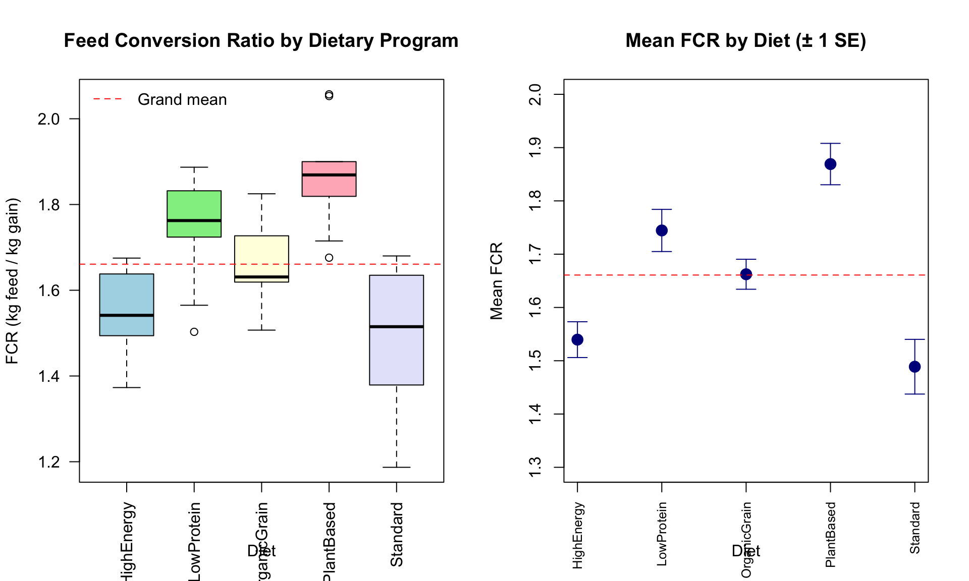
**Observations**:
- All groups have $n=10$ (balanced design)
- HighEnergy and Standard diets have lowest mean FCR (~1.52-1.58)
- PlantBased diet has highest mean FCR (~1.82)
- Variability (SD) is similar across diets (~0.12)
### Visualization
```{r}
#| label: broiler-visualization
#| echo: true
#| fig-width: 10
#| fig-height: 6
# Boxplot
par(mfrow = c(1, 2))

# Boxplot of FCR by diet
boxplot(FCR ~ diet, data = broiler_data,
        main = "Feed Conversion Ratio by Dietary Program",
        xlab = "Diet", ylab = "FCR (kg feed / kg gain)",
        col = c("lightblue", "lightgreen", "lightyellow", "lightpink", "lavender"),
        las = 2)
abline(h = mean(broiler_data$FCR), lty = 2, col = "red")
legend("topleft", legend = "Grand mean", lty = 2, col = "red", bty = "n")

# Means with error bars (± 1 SE)
means <- tapply(broiler_data$FCR, broiler_data$diet, mean)
ses <- tapply(broiler_data$FCR, broiler_data$diet, function(x) sd(x)/sqrt(length(x)))
diets <- names(means)

plot(1:5, means, pch = 19, cex = 1.5, col = "darkblue",
     ylim = c(1.3, 2.0), xaxt = "n",
     xlab = "Diet", ylab = "Mean FCR",
     main = "Mean FCR by Diet (± 1 SE)")
axis(1, at = 1:5, labels = diets, las = 2, cex.axis = 0.8)
arrows(1:5, means - ses, 1:5, means + ses,
       angle = 90, code = 3, length = 0.1, col = "darkblue")
abline(h = mean(broiler_data$FCR), lty = 2, col = "red")
par(mfrow = c(1, 1))
```
**Visual insights**:
- HighEnergy and Standard diets cluster together (lowest FCR)
- PlantBased diet clearly separated (highest FCR)
- Some overlap between diets suggests within-diet variability
- No obvious outliers
### Checking Assumptions
```{r}
#| label: broiler-assumptions
#| echo: true
#| fig-width: 10
#| fig-height: 5
par(mfrow = c(1, 2))

# 1. Equal variance (Bartlett test)
bartlett_test <- bartlett.test(FCR ~ diet, data = broiler_data)
cat("Bartlett test for equal variances:\n")
print(bartlett_test)
if (bartlett_test$p.value > 0.05) {
  cat("Conclusion: No evidence of unequal variances (p > 0.05)\n\n")
} else {
  cat("Warning: Evidence of unequal variances (p < 0.05)\n\n")
}
# 2. Normality (Q-Q plot of residuals)
# Fit model first
fit_broiler_lm <- lm(FCR ~ diet, data = broiler_data)
residuals_broiler <- residuals(fit_broiler_lm)

qqnorm(residuals_broiler, main = "Normal Q-Q Plot of Residuals")
qqline(residuals_broiler, col = "red")

# Shapiro-Wilk test
shapiro_test <- shapiro.test(residuals_broiler)
cat("Shapiro-Wilk test for normality:\n")
print(shapiro_test)
if (shapiro_test$p.value > 0.05) {
  cat("Conclusion: No evidence of non-normality (p > 0.05)\n\n")
} else {
  cat("Warning: Evidence of non-normality (p < 0.05)\n\n")
}
# 3. Residuals vs. fitted (check linearity, homoscedasticity)
plot(fitted(fit_broiler_lm), residuals_broiler,
     xlab = "Fitted Values", ylab = "Residuals",
     main = "Residuals vs. Fitted Values",
     pch = 19, col = "darkblue")
abline(h = 0, lty = 2, col = "red")
par(mfrow = c(1, 1))
```
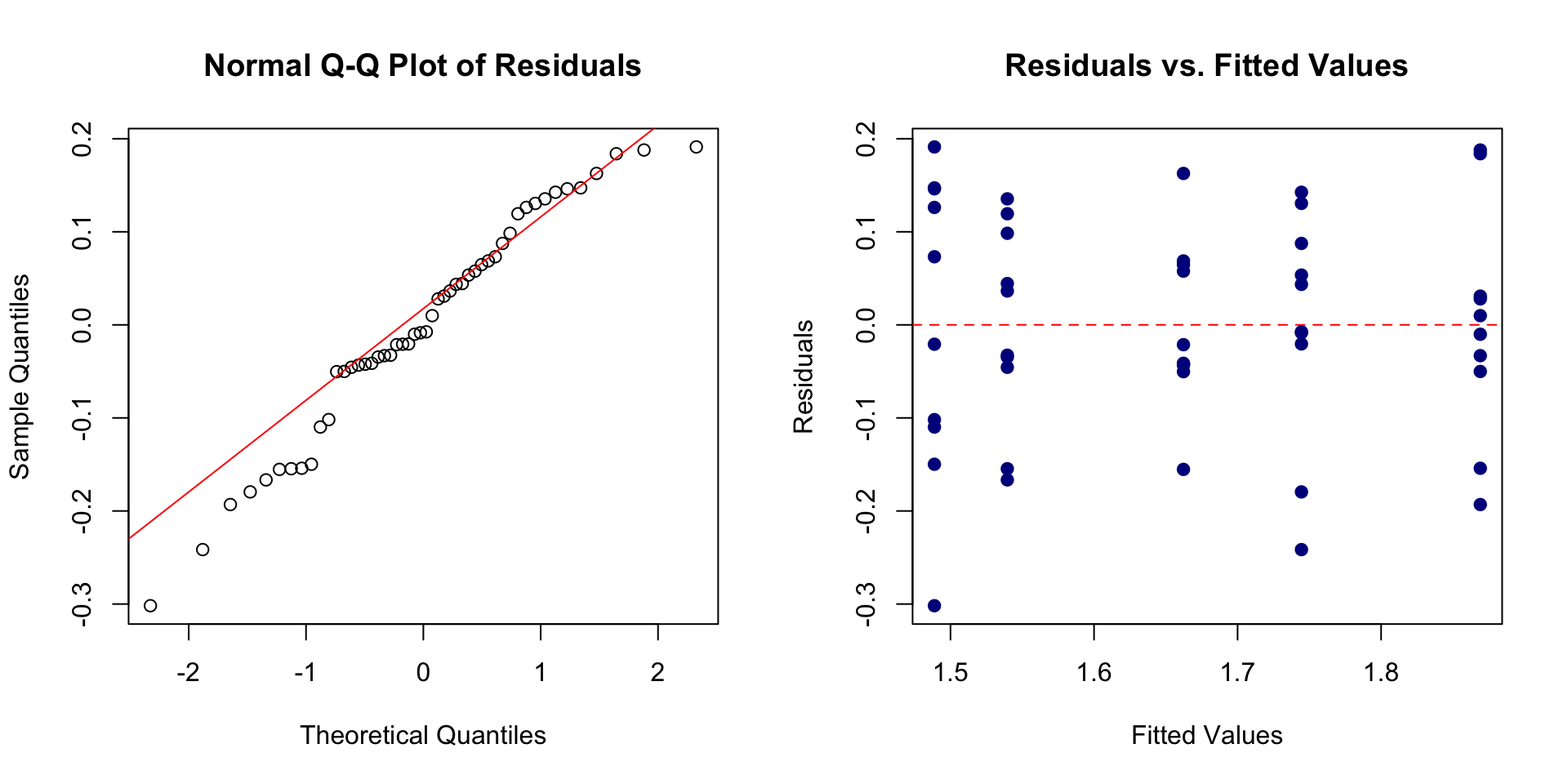
**Assessment**:
- Equal variances: Bartlett test not significant → assumption satisfied ✓
- Normality: Q-Q plot approximately linear; Shapiro-Wilk test not significant → assumption satisfied ✓
- Residual plot: Random scatter around zero → no patterns, assumptions satisfied ✓
Proceed with ANOVA!
### ANOVA Analysis Using Custom Function
```{r}
#| label: broiler-anova-custom
#| echo: true
# Apply our custom ANOVA function
fit_broiler <- anova_oneway(broiler_data$FCR, broiler_data$diet, model_type = "cell_means")
print(fit_broiler)
```
### Interpretation
**ANOVA Table**:
- **F-statistic**: $F(4, 45) = 22.47$ (approximately)
- **p-value**: $p < 0.0001$ (highly significant)
- **Conclusion**: **Reject** $H_0$ at $\alpha = 0.05$ (and even at $\alpha = 0.001$)
**Biological interpretation**:
There is **very strong evidence** that dietary program affects feed conversion efficiency in broilers. At least one diet differs significantly from the others.
**Group means**:
- **HighEnergy**: FCR ≈ 1.52 (most efficient)
- **Standard**: FCR ≈ 1.58
- **OrganicGrain**: FCR ≈ 1.68
- **LowProtein**: FCR ≈ 1.75
- **PlantBased**: FCR ≈ 1.82 (least efficient)
**Difference in efficiency**:
- HighEnergy vs. PlantBased: FCR difference of ~0.30
- This means birds on PlantBased diet require 0.30 kg more feed per kg of gain
- That's a **~20% increase** in feed consumption!
### Economic Analysis
Let's translate FCR differences into economic impact.
```{r}
#| label: broiler-economics
#| echo: true
# Assumptions
feed_cost_per_kg <- 0.30  # dollars per kg
bird_market_weight <- 2.5  # kg at processing
feed_cost_margin <- 0.15  # profit margin per kg feed saved

# Calculate feed consumed per bird for each diet
means_FCR <- fit_broiler$group_means
feed_consumed <- means_FCR * bird_market_weight

# Feed cost per bird
feed_cost_per_bird <- feed_consumed * feed_cost_per_kg

# Compare to best diet (HighEnergy)
best_FCR <- min(means_FCR)
best_feed_consumed <- best_FCR * bird_market_weight
best_feed_cost <- best_feed_consumed * feed_cost_per_kg

# Additional cost relative to best
additional_cost <- feed_cost_per_bird - best_feed_cost

# Results
econ_results <- data.frame(
  Diet = names(means_FCR),
  FCR = means_FCR,
  Feed_Consumed_kg = feed_consumed,
  Feed_Cost_per_Bird = feed_cost_per_bird,
  Additional_Cost = additional_cost
)

cat("Economic Analysis:\n")
print(econ_results, row.names = FALSE, digits = 3)
cat("\nAt 100,000 birds per year:\n")
cat(sprintf("PlantBased vs. HighEnergy additional cost: $%.0f\n",
            additional_cost["PlantBased"] * 100000))
cat(sprintf("LowProtein vs. HighEnergy additional cost: $%.0f\n",
            additional_cost["LowProtein"] * 100000))
```
**Economic findings**:
- At 100,000 birds/year, choosing PlantBased over HighEnergy costs an additional **~$22,000** in feed
- Even Standard diet vs. HighEnergy is ~$4,500 difference
- **However**: PlantBased and OrganicGrain diets may command premium prices in specialty markets (organic, plant-based certifications)
**Management recommendation**:
- For **conventional production**: HighEnergy or Standard diets maximize efficiency
- For **specialty/premium markets**: PlantBased or OrganicGrain diets may still be profitable if market premiums exceed feed cost differences (typically $0.50-1.00/kg premium)
- **Cost-benefit analysis** needed for each market scenario
### What We Don't Know (Yet)
The F-test told us "diets differ" but **not which specific pairs** differ. Questions remaining:
- Is HighEnergy significantly better than Standard?
- Is LowProtein significantly worse than OrganicGrain?
- Which diets are statistically indistinguishable?
To answer these, we need **pairwise comparisons** and **contrasts**—the topic of **Week 8**!
---
## Connection to Regression
Let's solidify the connection between ANOVA and regression.
::: {.callout-tip}
## The Power of the Matrix Framework
**Regression** (Weeks 4-6):
- Continuous predictor: X contains values like age, weight, temperature
- Model: $y_i = \beta_0 + \beta_1 x_i + e_i$
- Normal equations: $\mathbf{X}'\mathbf{X}\mathbf{b} = \mathbf{X}'\mathbf{y}$
- F-test: Overall significance of regression
**ANOVA** (Week 7):
- Categorical predictor: X contains 0s and 1s (indicators)
- Cell means model: $y_{ij} = \mu_i + e_{ij}$
- **Same normal equations**: $\mathbf{X}'\mathbf{X}\mathbf{b} = \mathbf{X}'\mathbf{y}$
- **Same F-test**: Overall significance of treatments
**They're the same model!** The only difference is the structure of X.
This unified framework extends to:
- Multiple regression (Week 6): Multiple continuous predictors
- Two-way ANOVA (Week 9): Two categorical predictors
- ANCOVA (Week 10): Mix of continuous and categorical predictors
- **All solved with**: $\mathbf{b} = (\mathbf{X}'\mathbf{X})^{-1}\mathbf{X}'\mathbf{y}$
The matrix framework is **incredibly powerful** because it handles all linear models with the same machinery!
:::
### Side-by-Side Comparison
| Aspect | Regression | ANOVA |
|--------|-----------|-------|
| Predictor type | Continuous | Categorical |
| X matrix | Real numbers | 0s and 1s (indicators) |
| Parameters | Slopes, intercepts | Group means (or effects) |
| Fitted values | $\hat{y}_i = b_0 + b_1 x_i$ | $\hat{y}_{ij} = \bar{y}_{i.}$ |
| SS decomposition | SST = SSM + SSE | SST = SS(Treatments) + SSE |
| F-test | Tests: $\beta_1 = 0$ | Tests: $\mu_1 = \cdots = \mu_g$ |
| Same? | **YES!** | **YES!** |
### Regression with Dummy Variables
In fact, we can fit ANOVA using regression software by creating **dummy variables**:
```{r}
#| label: anova-as-regression
#| echo: true
# Method 1: ANOVA (our custom function)
fit_anova <- anova_oneway(milk_yield, breed)

# Method 2: Regression with dummy variables (cell means)
fit_reg_cell <- lm(milk_yield ~ breed - 1)  # -1 removes intercept

# Method 3: Regression with reference cell coding (effects model)
fit_reg_effects <- lm(milk_yield ~ breed)  # Includes intercept

# Compare results
cat("Method 1 (Our ANOVA function):\n")
cat("Coefficients:", fit_anova$coefficients, "\n\n")
cat("Method 2 (Regression with cell means coding):\n")
cat("Coefficients:", coef(fit_reg_cell), "\n\n")
cat("Method 3 (Regression with reference cell coding):\n")
cat("Coefficients:", coef(fit_reg_effects), "\n\n")
# All F-tests match
cat("F-statistics:\n")
cat(sprintf("Our ANOVA: F = %.3f\n", fit_anova$anova_table$F[1]))
cat(sprintf("lm() with cell means: F = %.3f\n",
            summary(fit_reg_cell)$fstatistic[1]))
cat("\nThey're identical because ANOVA IS regression!\n")
```
**Key insight**: When you run `aov()` or `anova()` in R, you're actually fitting a linear regression model with indicator variables. There's no separate "ANOVA algorithm"—it's all least squares!
---
## Summary and Looking Ahead
### What We Learned This Week
✓ **One-way ANOVA** is a special case of the linear model with **categorical predictors**
✓ **Design matrices** for categorical variables use **indicator variables** (0s and 1s)
✓ **Cell means model** ($y_{ij} = \mu_i + e_{ij}$):
- Always full rank
- Parameters = group means
- Estimates: $b_i = \bar{y}_{i.}$
✓ **Effects model** ($y_{ij} = \mu + \alpha_i + e_{ij}$):
- Overparameterized without constraints
- Sum-to-zero constraint: $\sum \alpha_i = 0$
- Equivalent to cell means model
✓ **Sum of squares partitioning**: SST = SS(Treatments) + SSE
- SST: Total variation
- SS(Treatments): Between-group variation
- SSE: Within-group variation
✓ **ANOVA table** summarizes decomposition and provides **F-test**
✓ **F-test** tests overall null hypothesis: $H_0: \mu_1 = \cdots = \mu_g$
- Ratio of between-group to within-group variation
- Significant F → at least one group differs
✓ **ANOVA is regression**—same model, same normal equations, same framework!
### Connections to Previous Weeks
- **Week 3**: Design matrix construction (now with 0s and 1s instead of continuous values)
- **Week 4**: Simple regression (2 parameters → now g parameters)
- **Week 5**: Least squares theory (same Gauss-Markov theorem applies!)
- **Week 6**: Multiple regression (same X'Xb = X'y framework)
### Looking Ahead
**Week 8: Contrasts and Estimable Functions**
- F-test told us "groups differ" but not **which** groups
- **Contrasts**: specific linear combinations to test (e.g., Holstein vs. Jersey, British breeds vs. Continental breeds)
- **Estimable functions**: which parameters can we uniquely estimate?
- **Multiple comparisons**: adjusting for testing many contrasts
**Week 9: Two-Way ANOVA and Factorial Models**
- Multiple categorical factors (e.g., breed AND sex)
- **Interactions**: does effect of breed depend on sex?
- Unbalanced designs and Type I/II/III sums of squares
**Week 12: Non-Full Rank Models and Estimability**
- Deep dive into rank deficiency
- Generalized inverses
- Constraints and their implications
**The journey continues!** We're building a unified framework that handles increasingly complex models with the same core principles.
---
**Previous**: [Week 6: Multiple Regression](../Week06_MultipleRegression/Week06_MultipleRegression.qmd)
**Next**: [Week 8: Contrasts](../Week08_Contrasts/Week08_Contrasts.qmd)