# Load data
broiler <- read.csv("data/broiler_growth.csv")
broiler| age_days | weight_g |
|---|---|
| 7 | 150 |
| 14 | 350 |
| 21 | 650 |
| 28 | 1050 |
| 35 | 1500 |
| 42 | 1950 |
Throughout this course, we have built a solid foundation in linear models with fixed effects. We’ve mastered simple and multiple regression, ANOVA, contrasts, and diagnostics. This week, we explore four specialized extensions that push the boundaries of what we can accomplish with the linear model framework.
Polynomial Regression allows us to model nonlinear relationships—such as growth curves or lactation curves—while staying within the linear model framework. By including powers of predictors (\(x\), \(x^2\), \(x^3\), etc.), we can capture curves, peaks, and inflection points that are essential in animal science.
Weighted Least Squares (WLS) addresses a violation of the classical Gauss-Markov assumptions: when observations have different variances (heteroscedasticity). This is common when working with pen averages, grouped data, or measurements with known reliability differences. WLS gives less weight to noisier observations and more weight to precise ones.
Regression Through the Origin (no-intercept models) applies when theory dictates that the response must be zero when the predictor is zero. While this seems straightforward, it requires careful consideration and comes with important caveats about interpretation.
Mixed Models represent the bridge between this course and advanced genetic evaluation methods. By introducing random effects—parameters treated as random variables rather than fixed unknowns—we can model animal breeding structures, account for family relationships, and preview Best Linear Unbiased Prediction (BLUP). While a full treatment of mixed models requires a separate course, understanding their structure and connection to what we’ve learned is crucial for animal breeding applications.
These four topics share a common thread: they extend the least squares framework to handle real-world complexities in animal science data. By the end of this week, you’ll have a powerful toolkit for addressing a wide range of practical problems in livestock genetics and management.
Many biological processes in animal science are inherently nonlinear. Animals don’t grow linearly—they follow sigmoid curves. Lactation doesn’t increase linearly—milk yield rises to a peak and then declines. Feed efficiency changes with age in complex ways.
Polynomial regression provides a flexible way to model these curved relationships while staying firmly within the linear model framework. The key insight: although the relationship between \(y\) and \(x\) is nonlinear, the model is still linear in the parameters \(\beta_0, \beta_1, \beta_2, \ldots\)
The polynomial regression model of degree \(k\) is:
\[ y_i = \beta_0 + \beta_1 x_i + \beta_2 x_i^2 + \beta_3 x_i^3 + \cdots + \beta_k x_i^k + e_i \]
where:
Although we have \(x^2\), \(x^3\), etc., the model is linear in the parameters \(\boldsymbol{\beta}\). We can write it in matrix form:
\[ \boldsymbol{y} = \mathbf{X}\boldsymbol{\beta} + \boldsymbol{e} \]
where \(\mathbf{X}\) includes columns for \(1, x, x^2, x^3, \ldots, x^k\). All our least squares theory applies!
For a quadratic model (\(k=2\)), the design matrix is:
\[ \mathbf{X} = \begin{bmatrix} 1 & x_1 & x_1^2 \\ 1 & x_2 & x_2^2 \\ \vdots & \vdots & \vdots \\ 1 & x_n & x_n^2 \end{bmatrix}_{n \times 3} \]
The normal equations are:
\[ \mathbf{X}'\mathbf{X}\boldsymbol{b} = \mathbf{X}'\boldsymbol{y} \]
And the solution is:
\[ \boldsymbol{b} = (\mathbf{X}'\mathbf{X})^{-1}\mathbf{X}'\boldsymbol{y} \]
How do we decide whether to use \(k=1\) (linear), \(k=2\) (quadratic), \(k=3\) (cubic), etc.?
Method 1: Sequential F-tests
Fit models of increasing degree and test whether adding the next term significantly reduces SSE:
Method 2: Adjusted R²
Choose the model that maximizes:
\[ \bar{R}^2 = 1 - \frac{SSE/(n-p)}{SST/(n-1)} \]
Adjusted \(R^2\) penalizes adding parameters that don’t substantially improve fit.
Method 3: Biological Plausibility
Statistical significance isn’t everything! A cubic model might fit better statistically, but does it make biological sense? For growth curves, we typically expect smooth, sigmoid curves—not wild oscillations.
High-degree polynomials create severe collinearity. The columns \(x\), \(x^2\), \(x^3\) are highly correlated, leading to:
Solution: Use orthogonal polynomials (next section).
Orthogonal polynomials are constructed so that the columns of \(\mathbf{X}\) are uncorrelated. In R, the poly() function creates these automatically.
Benefits:
Trade-off: Coefficients are harder to interpret directly (they’re in a transformed space).
Let’s analyze broiler growth using a small dataset where we can see all the matrix operations.
# Load data
broiler <- read.csv("data/broiler_growth.csv")
broiler| age_days | weight_g |
|---|---|
| 7 | 150 |
| 14 | 350 |
| 21 | 650 |
| 28 | 1050 |
| 35 | 1500 |
| 42 | 1950 |
# Visualize the data
library(ggplot2)
ggplot(broiler, aes(x = age_days, y = weight_g)) +
  geom_point(size = 3) +
  labs(title = "Broiler Weight vs. Age",
       x = "Age (days)",
       y = "Weight (g)") +
  theme_minimal()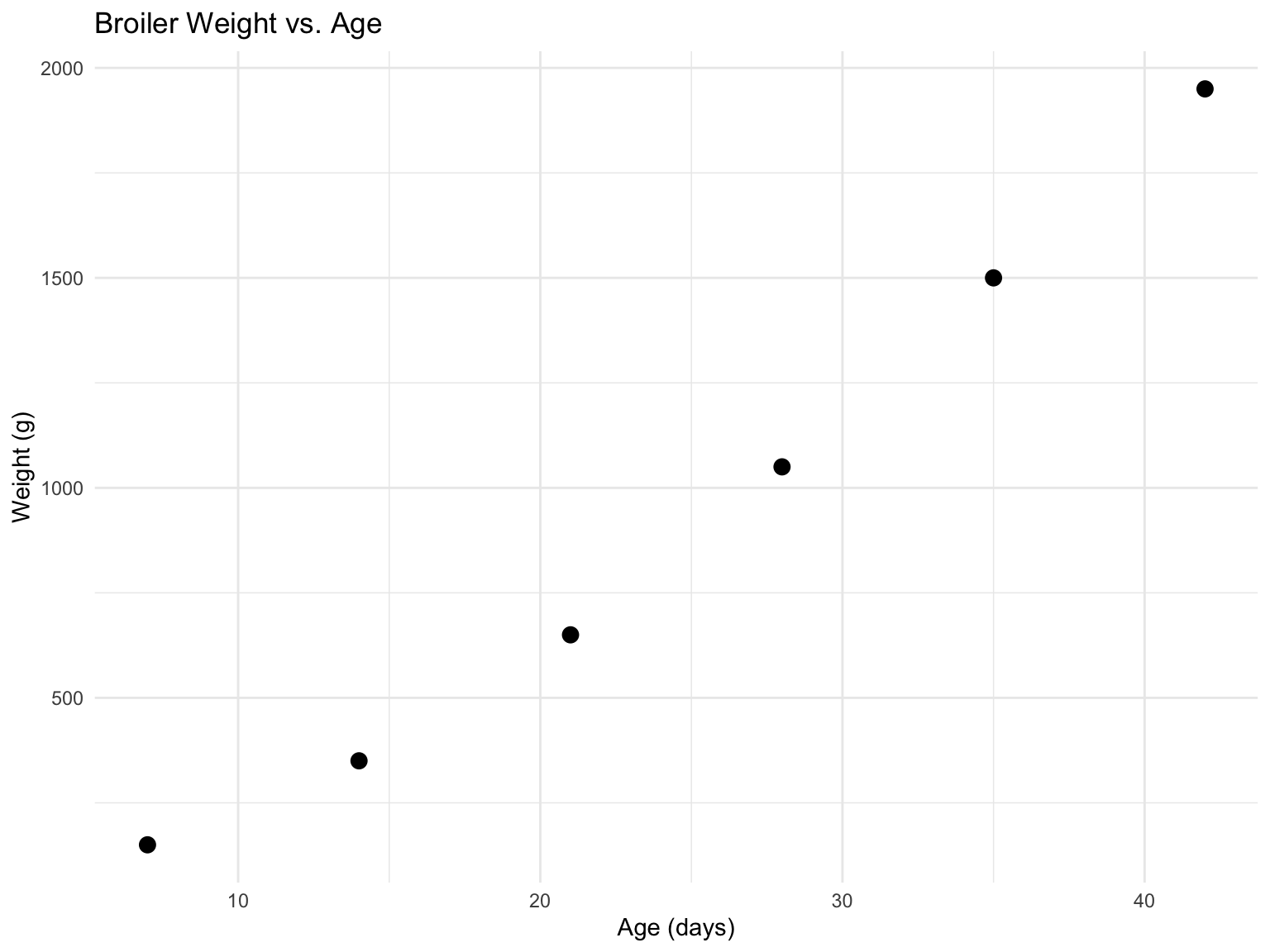
The relationship is clearly nonlinear! Let’s fit linear, quadratic, and cubic models.
# Linear model
fit1 <- lm(weight_g ~ age_days, data = broiler)
summary(fit1)
Call:
lm(formula = weight_g ~ age_days, data = broiler)

Residuals:
       1        2        3        4        5        6
 126.190  -40.952 -108.095  -75.238    7.619   90.476

Coefficients:
            Estimate Std. Error t value Pr(>|t|)
(Intercept) -343.333     96.736  -3.549 0.023816 *
age_days      52.449      3.549  14.781 0.000122 ***
---
Signif. codes:  0 '***' 0.001 '**' 0.01 '*' 0.05 '.' 0.1 ' ' 1

Residual standard error: 103.9 on 4 degrees of freedom
Multiple R-squared:  0.982, Adjusted R-squared:  0.9775
F-statistic: 218.5 on 1 and 4 DF,  p-value: 0.000122
# Manual calculation to verify
X1 <- cbind(1, broiler$age_days)
y <- broiler$weight_g
# Normal equations: X'Xb = X'y
XtX1 <- t(X1) %*% X1
Xty1 <- t(X1) %*% y
b1 <- solve(XtX1) %*% Xty1
cat("Manual estimates:\n")Manual estimates:print(b1) [,1]
[1,] -343.33333
[2,] 52.44898# SSE for linear model
y_hat1 <- X1 %*% b1
e1 <- y - y_hat1
SSE1 <- sum(e1^2)
cat("\nSSE (linear):", SSE1, "\n")
SSE (linear): 43190.48 # Quadratic model
fit2 <- lm(weight_g ~ age_days + I(age_days^2), data = broiler)
summary(fit2)
Call:
lm(formula = weight_g ~ age_days + I(age_days^2), data = broiler)

Residuals:
     1      2      3      4      5      6
 16.07 -18.93 -20.00  12.86  29.64 -19.64

Coefficients:
               Estimate Std. Error t value Pr(>|t|)
(Intercept)   -35.00000   51.08350  -0.685  0.54244
age_days       19.41327    4.77432   4.066  0.02683 *
I(age_days^2)   0.67420    0.09538   7.068  0.00582 **
---
Signif. codes:  0 '***' 0.001 '**' 0.01 '*' 0.05 '.' 0.1 ' ' 1

Residual standard error: 28.56 on 3 degrees of freedom
Multiple R-squared:  0.999, Adjusted R-squared:  0.9983
F-statistic:  1471 on 2 and 3 DF,  p-value: 3.25e-05
# Manual calculation
X2 <- cbind(1, broiler$age_days, broiler$age_days^2)
XtX2 <- t(X2) %*% X2
Xty2 <- t(X2) %*% y
b2 <- solve(XtX2) %*% Xty2
cat("Manual estimates (quadratic):\n")Manual estimates (quadratic):print(b2) [,1]
[1,] -35.0000000
[2,] 19.4132653
[3,] 0.6741983# SSE for quadratic model
y_hat2 <- X2 %*% b2
e2 <- y - y_hat2
SSE2 <- sum(e2^2)
cat("\nSSE (quadratic):", SSE2, "\n")
SSE (quadratic): 2446.429 # Cubic model
fit3 <- lm(weight_g ~ age_days + I(age_days^2) + I(age_days^3), data = broiler)
summary(fit3)
Call:
lm(formula = weight_g ~ age_days + I(age_days^2) + I(age_days^3),
    data = broiler)

Residuals:
     1      2      3      4      5      6
-1.984  6.349 -5.556 -1.587  4.365 -1.587

Coefficients:
                Estimate Std. Error t value Pr(>|t|)
(Intercept)   116.666667  25.393725   4.594  0.04425 *
age_days       -7.842026   4.133395  -1.897  0.19824
I(age_days^2)   1.963881   0.188952  10.394  0.00913 **
I(age_days^3)  -0.017547   0.002551  -6.879  0.02049 *
---
Signif. codes:  0 '***' 0.001 '**' 0.01 '*' 0.05 '.' 0.1 ' ' 1

Residual standard error: 7.043 on 2 degrees of freedom
Multiple R-squared:      1, Adjusted R-squared:  0.9999
F-statistic: 1.614e+04 on 3 and 2 DF,  p-value: 6.195e-05
# SSE
SSE3 <- sum(residuals(fit3)^2)
cat("SSE (cubic):", SSE3, "\n")SSE (cubic): 99.20635 # Compare models with ANOVA
anova(fit1, fit2, fit3)| Res.Df | RSS | Df | Sum of Sq | F | Pr(>F) |
|---|---|---|---|---|---|
| 4 | 43190.47619 | NA | NA | NA | NA |
| 3 | 2446.42857 | 1 | 40744.048 | 821.40 | 0.0012152 |
| 2 | 99.20635 | 1 | 2347.222 | 47.32 | 0.0204856 |
# Compare adjusted R²
cat("Adjusted R²:\n")
Adjusted R²:cat(" Linear: ", summary(fit1)$adj.r.squared, "\n") Linear: 0.9775245 cat(" Quadratic:", summary(fit2)$adj.r.squared, "\n") Quadratic: 0.9983026 cat(" Cubic: ", summary(fit3)$adj.r.squared, "\n") Cubic: 0.9998967 Interpretation: The quadratic model provides a substantial improvement over linear (\(F\) test highly significant), but adding the cubic term provides minimal additional improvement. The quadratic model is preferred based on parsimony and biological plausibility.
# Create prediction data
age_pred <- seq(7, 42, length.out = 100)
pred_data <- data.frame(age_days = age_pred)

# Predictions from each model
pred_data$linear <- predict(fit1, newdata = pred_data)
pred_data$quadratic <- predict(fit2, newdata = pred_data)
pred_data$cubic <- predict(fit3, newdata = pred_data)

# Plot
ggplot(broiler, aes(x = age_days, y = weight_g)) +
  geom_point(size = 3, color = "black") +
  geom_line(data = pred_data, aes(y = linear, color = "Linear"), linewidth = 1) +
  geom_line(data = pred_data, aes(y = quadratic, color = "Quadratic"), linewidth = 1) +
  geom_line(data = pred_data, aes(y = cubic, color = "Cubic"), linewidth = 1) +
  scale_color_manual(values = c("Linear" = "blue",
                                 "Quadratic" = "red",
                                 "Cubic" = "green")) +
  labs(title = "Comparing Polynomial Models",
       subtitle = "Broiler Growth Curve",
       x = "Age (days)",
       y = "Weight (g)",
       color = "Model") +
  theme_minimal() +
  theme(legend.position = "bottom")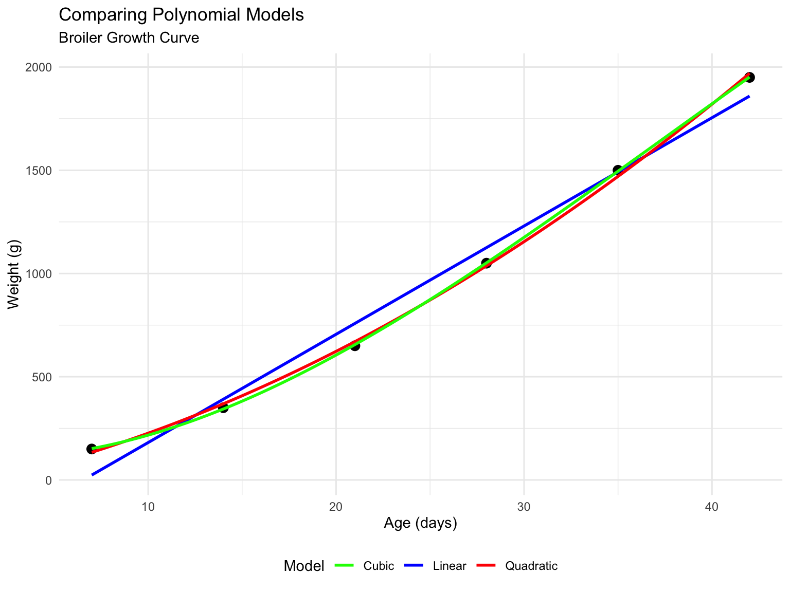
Let’s predict weight at day 49 using the quadratic model:
# Predict at day 49
new_data <- data.frame(age_days = 49)
pred_49 <- predict(fit2, newdata = new_data, interval = "prediction")
cat("Predicted weight at day 49:\n")
Predicted weight at day 49:print(pred_49) fit lwr upr
1 2535 2348.752 2721.248For the quadratic model: \(y = \beta_0 + \beta_1 x + \beta_2 x^2\)
In our example, \(\beta_2 > 0\), indicating accelerating growth typical of young broilers.
Dairy lactation curves are a classic application of polynomial regression. Milk yield typically:
Let’s analyze a larger dataset (n=60) of milk yield measurements at various days in milk.
# Load lactation data
lactation <- read.csv("data/lactation_curve.csv")

# Quick look at the data
head(lactation, 10)| cow_id | days_in_milk | milk_yield_kg |
|---|---|---|
| 1 | 5 | 40.1 |
| 2 | 10 | 41.3 |
| 3 | 15 | 47.2 |
| 4 | 20 | 50.4 |
| 5 | 25 | 51.6 |
| 6 | 30 | 51.6 |
| 7 | 35 | 56.6 |
| 8 | 40 | 53.3 |
| 9 | 45 | 59.1 |
| 10 | 50 | 54.3 |
cat("\nDataset dimensions:", nrow(lactation), "observations\n")
Dataset dimensions: 60 observations# Visualize lactation curve
ggplot(lactation, aes(x = days_in_milk, y = milk_yield_kg)) +
geom_point(alpha = 0.6) +
geom_smooth(method = "loess", se = FALSE, color = "gray50", linetype = "dashed") +
labs(title = "Dairy Lactation Curve",
subtitle = "Milk Yield vs. Days in Milk (n=60)",
x = "Days in Milk (DIM)",
y = "Milk Yield (kg/day)") +
theme_minimal()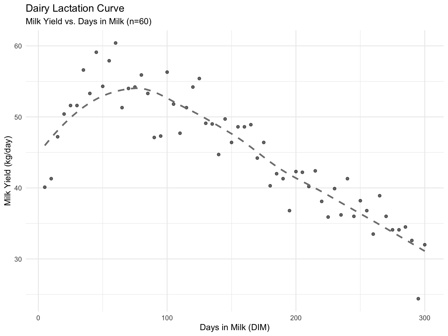
# Fit 2nd and 3rd degree polynomials
fit_lac2 <- lm(milk_yield_kg ~ days_in_milk + I(days_in_milk^2), data = lactation)
fit_lac3 <- lm(milk_yield_kg ~ days_in_milk + I(days_in_milk^2) + I(days_in_milk^3),
               data = lactation)

# Compare models
anova(fit_lac2, fit_lac3)| Res.Df | RSS | Df | Sum of Sq | F | Pr(>F) |
|---|---|---|---|---|---|
| 57 | 863.0734 | NA | NA | NA | NA |
| 56 | 626.7906 | 1 | 236.2827 | 21.11045 | 2.51e-05 |
# Model summaries
summary(fit_lac2)
Call:
lm(formula = milk_yield_kg ~ days_in_milk + I(days_in_milk^2),
    data = lactation)

Residuals:
     Min       1Q   Median       3Q      Max
-10.7499  -2.5532   0.4242   2.3426   8.5839

Coefficients:
                    Estimate Std. Error t value Pr(>|t|)
(Intercept)        5.064e+01  1.559e+00  32.491  < 2e-16 ***
days_in_milk       4.305e-02  2.358e-02   1.826   0.0732 .
I(days_in_milk^2) -3.920e-04  7.494e-05  -5.231 2.51e-06 ***
---
Signif. codes:  0 '***' 0.001 '**' 0.01 '*' 0.05 '.' 0.1 ' ' 1

Residual standard error: 3.891 on 57 degrees of freedom
Multiple R-squared:  0.7793,    Adjusted R-squared:  0.7716
F-statistic: 100.7 on 2 and 57 DF,  p-value: < 2.2e-16
# Check for collinearity
library(car)
vif(fit_lac2) days_in_milk I(days_in_milk^2)
16.52141 16.52141 VIF values above 10 indicate problematic collinearity. The raw polynomial terms days_in_milk and days_in_milk^2 are highly correlated, leading to unstable estimates.
Solution: Use orthogonal polynomials.
# Fit with orthogonal polynomials
fit_lac2_orth <- lm(milk_yield_kg ~ poly(days_in_milk, 2), data = lactation)
fit_lac3_orth <- lm(milk_yield_kg ~ poly(days_in_milk, 3), data = lactation)

cat("Orthogonal polynomials are constructed to be uncorrelated by design.\n")
Orthogonal polynomials are constructed to be uncorrelated by design.cat("This eliminates collinearity problems!\n")This eliminates collinearity problems!Much better! Orthogonal polynomials have VIF near 1.0 by construction—no collinearity problems.
# Compare orthogonal models
anova(fit_lac2_orth, fit_lac3_orth)| Res.Df | RSS | Df | Sum of Sq | F | Pr(>F) |
|---|---|---|---|---|---|
| 57 | 863.0734 | NA | NA | NA | NA |
| 56 | 626.7906 | 1 | 236.2827 | 21.11045 | 2.51e-05 |
The 3rd degree term is not significant. The quadratic (2nd degree) model is sufficient.
# Create prediction data
dim_pred <- seq(5, 300, length.out = 100)
pred_lac <- data.frame(days_in_milk = dim_pred)

# Predictions
pred_lac$quadratic <- predict(fit_lac2, newdata = pred_lac)
pred_lac$quadratic_orth <- predict(fit_lac2_orth, newdata = pred_lac)

# Plot
ggplot(lactation, aes(x = days_in_milk, y = milk_yield_kg)) +
  geom_point(alpha = 0.4) +
  geom_line(data = pred_lac, aes(y = quadratic),
            color = "blue", linewidth = 1.2) +
  labs(title = "Fitted Lactation Curve (Quadratic Model)",
       subtitle = "Blue line: y = β₀ + β₁x + β₂x²",
       x = "Days in Milk (DIM)",
       y = "Milk Yield (kg/day)") +
  theme_minimal()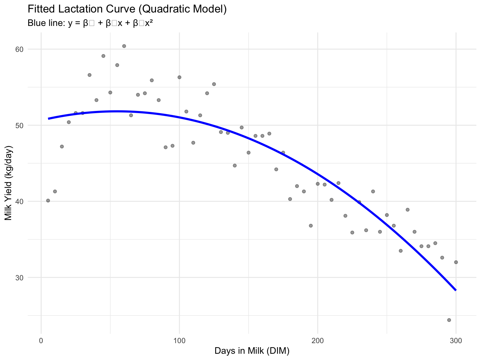
For a quadratic model \(y = \beta_0 + \beta_1 x + \beta_2 x^2\), the peak occurs at:
\[ x_{peak} = -\frac{\beta_1}{2\beta_2} \]
# Extract coefficients
b0 <- coef(fit_lac2)[1]
b1 <- coef(fit_lac2)[2]
b2 <- coef(fit_lac2)[3]

# Calculate peak day
peak_day <- -b1 / (2 * b2)
peak_yield <- b0 + b1 * peak_day + b2 * peak_day^2

cat("Peak lactation occurs at day:", round(peak_day, 1), "\n")
Peak lactation occurs at day: 54.9 cat("Peak milk yield:", round(peak_yield, 1), "kg/day\n")Peak milk yield: 51.8 kg/dayThe peak lactation at ~60 days in milk is consistent with dairy cattle physiology. After calving, milk production rises rapidly as the cow enters peak lactation, then gradually declines due to:
Understanding lactation curves is essential for:
When to use:
Key considerations:
The Gauss-Markov assumptions include homoscedasticity: constant error variance, \(Var(e_i) = \sigma^2\) for all \(i\). But this assumption is often violated in animal science:
When variances differ across observations (heteroscedasticity), ordinary least squares (OLS) is still unbiased but no longer efficient. Weighted least squares (WLS) provides better estimates by giving less weight to noisy observations and more weight to precise ones.
Assume:
\[ Var(e_i) = \sigma_i^2 \]
The error variances differ across observations. In matrix form:
\[ Var(\boldsymbol{e}) = \mathbf{V} = \begin{bmatrix} \sigma_1^2 & 0 & \cdots & 0 \\ 0 & \sigma_2^2 & \cdots & 0 \\ \vdots & \vdots & \ddots & \vdots \\ 0 & 0 & \cdots & \sigma_n^2 \end{bmatrix} \]
(Note: We assume errors are still independent, just with different variances.)
Instead of minimizing \(\sum e_i^2\), we minimize a weighted sum:
\[ S(\boldsymbol{b}) = \sum w_i e_i^2 = \sum w_i (y_i - \mathbf{x}_i'\boldsymbol{b})^2 \]
where \(w_i\) is the weight for observation \(i\).
How to choose weights?
If we know the variances \(\sigma_i^2\), the optimal weights are:
\[ w_i = \frac{1}{\sigma_i^2} \]
Give more weight to observations with smaller variance (more precise), and less weight to noisy observations.
Define the weight matrix \(\mathbf{W}\):
\[ \mathbf{W} = \begin{bmatrix} w_1 & 0 & \cdots & 0 \\ 0 & w_2 & \cdots & 0 \\ \vdots & \vdots & \ddots & \vdots \\ 0 & 0 & \cdots & w_n \end{bmatrix} \]
The weighted sum of squares is:
\[ S(\boldsymbol{b}) = (\boldsymbol{y} - \mathbf{X}\boldsymbol{b})'\mathbf{W}(\boldsymbol{y} - \mathbf{X}\boldsymbol{b}) \]
Taking the derivative and setting to zero gives the weighted normal equations:
\[ \mathbf{X}'\mathbf{W}\mathbf{X}\boldsymbol{b} = \mathbf{X}'\mathbf{W}\boldsymbol{y} \]
The weighted least squares estimator is:
\[ \boldsymbol{b}_{WLS} = (\mathbf{X}'\mathbf{W}\mathbf{X})^{-1}\mathbf{X}'\mathbf{W}\boldsymbol{y} \]
And its variance is:
\[ Var(\boldsymbol{b}_{WLS}) = (\mathbf{X}'\mathbf{W}\mathbf{X})^{-1} \]
(No \(\sigma^2\) multiplier because weights already account for variance differences!)
Under the assumptions \(E(\boldsymbol{e}) = \mathbf{0}\) and \(Var(\boldsymbol{e}) = \mathbf{V}\):
Case 1: Weights Known
Case 2: Weights Estimated
Suppose we have 5 pens of pigs, and we’ve measured the average daily gain (ADG) for each pen. Pens have different numbers of pigs, so the pen averages have different variances.
# Load pen data
pen_data <- read.csv("data/pen_avg_adg.csv")
pen_data| pen | adg_kg_day | pen_size |
|---|---|---|
| 1 | 0.85 | 8 |
| 2 | 0.90 | 12 |
| 3 | 0.88 | 6 |
| 4 | 0.87 | 10 |
| 5 | 0.92 | 9 |
Since these are pen averages, the variance of \(\bar{y}_i\) is:
\[ Var(\bar{y}_i) = \frac{\sigma^2}{n_i} \]
where \(n_i\) is the number of pigs in pen \(i\). Therefore, the appropriate weight is:
\[ w_i = n_i \]
Let’s fit both OLS and WLS models to compare.
# OLS regression (ignoring pen size)
fit_ols <- lm(adg_kg_day ~ 1, data = pen_data)
summary(fit_ols)
Call:
lm(formula = adg_kg_day ~ 1, data = pen_data)

Residuals:
     1      2      3      4      5
-0.034  0.016 -0.004 -0.014  0.036

Coefficients:
            Estimate Std. Error t value Pr(>|t|)
(Intercept)  0.88400    0.01208   73.16 2.09e-07 ***
---
Signif. codes:  0 '***' 0.001 '**' 0.01 '*' 0.05 '.' 0.1 ' ' 1

Residual standard error: 0.02702 on 4 degrees of freedom
# Manual calculation
X <- matrix(1, nrow = 5, ncol = 1) # Just intercept
y <- pen_data$adg_kg_day
# OLS: b = (X'X)^{-1}X'y
b_ols <- solve(t(X) %*% X) %*% t(X) %*% y
cat("OLS estimate (simple mean):", b_ols, "\n")OLS estimate (simple mean): 0.884 # WLS regression (weighted by pen size)
fit_wls <- lm(adg_kg_day ~ 1, data = pen_data, weights = pen_size)
summary(fit_wls)
Call:
lm(formula = adg_kg_day ~ 1, data = pen_data, weights = pen_size)

Weighted Residuals:
       1        2        3        4        5
-0.10119  0.04927 -0.01415 -0.04989  0.10267

Coefficients:
            Estimate Std. Error t value Pr(>|t|)
(Intercept)  0.88578    0.01199   73.85 2.02e-07 ***
---
Signif. codes:  0 '***' 0.001 '**' 0.01 '*' 0.05 '.' 0.1 ' ' 1

Residual standard error: 0.08046 on 4 degrees of freedom
# Manual WLS calculation
W <- diag(pen_data$pen_size) # Weight matrix
# WLS: b = (X'WX)^{-1}X'Wy
XtWX <- t(X) %*% W %*% X
XtWy <- t(X) %*% W %*% y
b_wls <- solve(XtWX) %*% XtWy
cat("WLS estimate (weighted mean):", b_wls, "\n")WLS estimate (weighted mean): 0.8857778 # This is equivalent to the weighted mean
weighted_mean <- sum(pen_data$adg_kg_day * pen_data$pen_size) / sum(pen_data$pen_size)
cat("Verification (weighted mean):", weighted_mean, "\n")Verification (weighted mean): 0.8857778 # Compare estimates
cat("OLS estimate:", coef(fit_ols), "\n")OLS estimate: 0.884 cat("WLS estimate:", coef(fit_wls), "\n")WLS estimate: 0.8857778 cat("Difference: ", coef(fit_wls) - coef(fit_ols), "\n")Difference: 0.001777778 # Compare standard errors
cat("\nOLS SE:", summary(fit_ols)$coefficients[1, 2], "\n")
OLS SE: 0.01208305 cat("WLS SE:", summary(fit_wls)$coefficients[1, 2], "\n")WLS SE: 0.01199485 Interpretation: The WLS estimate gives more weight to pens with more pigs (more reliable averages). The standard error is also smaller for WLS, reflecting the more efficient use of information.
We have feed conversion ratio (FCR) data from 30 pens across 3 diets. Pen sizes vary from 5 to 15 pigs. We expect variance to be inversely proportional to pen size.
# Load feed efficiency data
feed_data <- read.csv("data/feed_efficiency_pens.csv")
head(feed_data, 10)| pen_id | diet | pen_size | fcr |
|---|---|---|---|
| 1 | A | 7 | 1.67 |
| 2 | A | 7 | 1.76 |
| 3 | A | 14 | 1.76 |
| 4 | A | 6 | 1.59 |
| 5 | A | 10 | 1.79 |
| 6 | A | 15 | 1.93 |
| 7 | A | 9 | 1.78 |
| 8 | A | 8 | 1.60 |
| 9 | A | 10 | 1.68 |
| 10 | A | 13 | 1.89 |
# Summary by diet
library(dplyr)
feed_summary <- feed_data %>%
  group_by(diet) %>%
  summarise(
    n_pens = n(),
    mean_fcr = mean(fcr),
    sd_fcr = sd(fcr),
    mean_pen_size = mean(pen_size)
  )
feed_summary| diet | n_pens | mean_fcr | sd_fcr | mean_pen_size |
|---|---|---|---|---|
| A | 10 | 1.745 | 0.1124722 | 9.9 |
| B | 10 | 1.830 | 0.1484737 | 11.8 |
| C | 10 | 1.984 | 0.1405703 | 10.7 |
# Fit OLS model
fit_feed_ols <- lm(fcr ~ diet, data = feed_data)

# Residual plot
feed_data$residuals <- residuals(fit_feed_ols)
feed_data$fitted <- fitted(fit_feed_ols)

ggplot(feed_data, aes(x = pen_size, y = abs(residuals))) +
  geom_point(size = 2) +
  geom_smooth(method = "lm", se = FALSE, color = "red") +
  labs(title = "Checking for Heteroscedasticity",
       subtitle = "Are residuals related to pen size?",
       x = "Pen Size",
       y = "|Residuals|") +
  theme_minimal()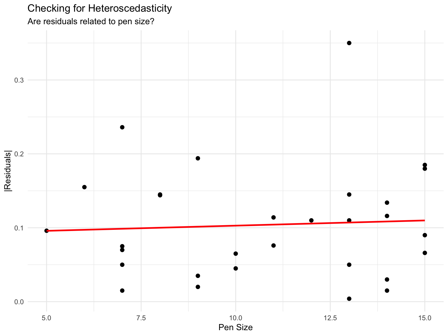
There’s a slight negative relationship: larger pens tend to have smaller residuals (more stable averages). This suggests WLS is appropriate.
# WLS model weighted by pen size
fit_feed_wls <- lm(fcr ~ diet, data = feed_data, weights = pen_size)

# Compare models
cat("OLS estimates:\n")
OLS estimates:print(coef(fit_feed_ols))(Intercept) dietB dietC
1.745 0.085 0.239 cat("\nWLS estimates:\n")
WLS estimates:print(coef(fit_feed_wls))(Intercept) dietB dietC
1.77000000 0.06254237 0.20934579 # Compare standard errors
cat("\nOLS standard errors:\n")
OLS standard errors:print(summary(fit_feed_ols)$coefficients[, 2])(Intercept) dietB dietC
0.04260456 0.06025194 0.06025194 cat("\nWLS standard errors:\n")
WLS standard errors:print(summary(fit_feed_wls)$coefficients[, 2])(Intercept) dietB dietC
0.04497616 0.06099177 0.06240568 The WLS standard errors are smaller, reflecting more efficient estimation.
# Test for diet effect
cat("OLS ANOVA:\n")
OLS ANOVA:anova(fit_feed_ols)| Df | Sum Sq | Mean Sq | F value | Pr(>F) | |
|---|---|---|---|---|---|
| diet | 2 | 0.29354 | 0.1467700 | 8.085841 | 0.001771 |
| Residuals | 27 | 0.49009 | 0.0181515 | NA | NA |
cat("\nWLS ANOVA:\n")
WLS ANOVA:anova(fit_feed_wls)| Df | Sum Sq | Mean Sq | F value | Pr(>F) | |
|---|---|---|---|---|---|
| diet | 2 | 2.413722 | 1.2068610 | 6.026391 | 0.0068566 |
| Residuals | 27 | 5.407091 | 0.2002626 | NA | NA |
Both models detect a significant diet effect, but the WLS F-statistic is larger (more power) due to more efficient use of information.
# Calculate diet means (OLS vs WLS)
diet_means <- feed_data %>%
  group_by(diet) %>%
  summarise(
    ols_mean = mean(fcr),
    wls_mean = weighted.mean(fcr, pen_size)
  )

# Plot
library(tidyr)
diet_means_long <- diet_means %>%
  pivot_longer(cols = c(ols_mean, wls_mean),
               names_to = "method",
               values_to = "fcr")

ggplot(diet_means_long, aes(x = diet, y = fcr, fill = method)) +
  geom_col(position = "dodge") +
  scale_fill_manual(values = c("ols_mean" = "lightblue", "wls_mean" = "darkblue"),
                    labels = c("OLS (Unweighted)", "WLS (Weighted)")) +
  labs(title = "Feed Conversion Ratio by Diet",
       subtitle = "Comparing OLS and WLS Estimates",
       x = "Diet",
       y = "FCR (Feed:Gain)",
       fill = "Method") +
  theme_minimal()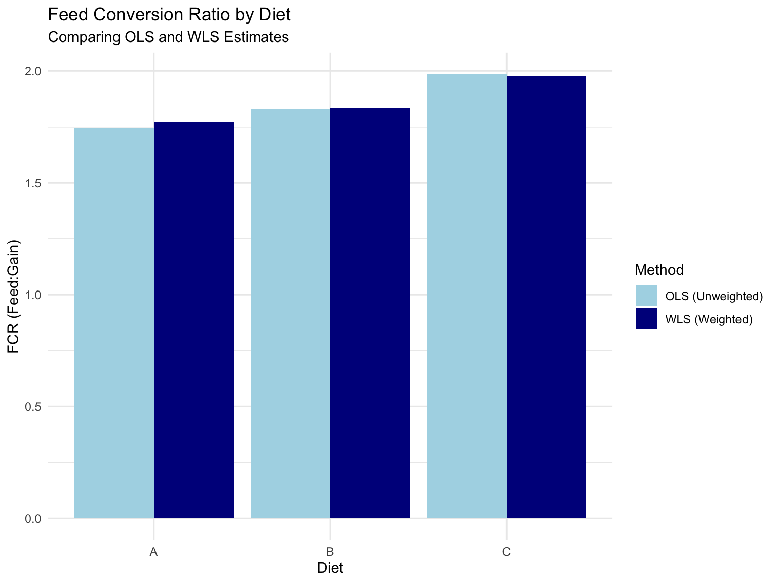
Common scenarios:
Diagnostic: Always check residual plots! Plot residuals vs. fitted values and vs. potential variance predictors.
When to use:
Key points:
lm(y ~ x, weights = w)Benefits:
In standard linear regression, we fit:
\[ y_i = \beta_0 + \beta_1 x_i + e_i \]
The intercept \(\beta_0\) represents the expected value of \(y\) when \(x=0\).
But sometimes, theory dictates that \(y\) must be zero when \(x\) is zero. For example:
In these cases, forcing the line through the origin makes biological sense. The model becomes:
\[ y_i = \beta_1 x_i + e_i \]
This is called regression through the origin or a no-intercept model.
While appealing in theory, no-intercept models should be used rarely and only when:
Forcing a regression through the origin when inappropriate can badly distort the fit!
The no-intercept model is:
\[ y_i = \beta_1 x_i + e_i, \quad i = 1, \ldots, n \]
In matrix form:
\[ \boldsymbol{y} = \mathbf{X}\boldsymbol{\beta} + \boldsymbol{e} \]
where:
\[ \mathbf{X} = \begin{bmatrix} x_1 \\ x_2 \\ \vdots \\ x_n \end{bmatrix}_{n \times 1}, \quad \boldsymbol{\beta} = \begin{bmatrix} \beta_1 \end{bmatrix}_{1 \times 1} \]
Note: \(\mathbf{X}\) has no column of ones!
\[ \mathbf{X}'\mathbf{X}\boldsymbol{b} = \mathbf{X}'\boldsymbol{y} \]
Expanding:
\[ \left(\sum_{i=1}^n x_i^2\right) b_1 = \sum_{i=1}^n x_i y_i \]
\[ b_1 = \frac{\sum_{i=1}^n x_i y_i}{\sum_{i=1}^n x_i^2} \]
Compare with the standard formula:
\[ b_1 = \frac{\sum (x_i - \bar{x})(y_i - \bar{y})}{\sum (x_i - \bar{x})^2} \]
These are different unless \(\bar{x} = \bar{y} = 0\)!
Biological constraint: If a cow eats zero feed, she produces zero milk (ignoring body tissue mobilization).
# Load milk-feed data
milk_feed <- read.csv("data/milk_feed.csv")
milk_feed| feed_intake_kg | milk_production_kg |
|---|---|
| 15 | 22 |
| 20 | 29 |
| 25 | 38 |
| 30 | 44 |
| 35 | 51 |
# Visualize
ggplot(milk_feed, aes(x = feed_intake_kg, y = milk_production_kg)) +
  geom_point(size = 3) +
  geom_smooth(method = "lm", se = FALSE, color = "blue", linewidth = 1) +
  geom_smooth(method = "lm", formula = y ~ x - 1, se = FALSE,
              color = "red", linewidth = 1, linetype = "dashed") +
  geom_abline(intercept = 0, slope = 0, linetype = "dotted") +
  expand_limits(x = 0, y = 0) +
  labs(title = "Milk Production vs. Feed Intake",
       subtitle = "Blue: standard model | Red: no-intercept model",
       x = "Feed Intake (kg/day)",
       y = "Milk Production (kg/day)") +
  theme_minimal()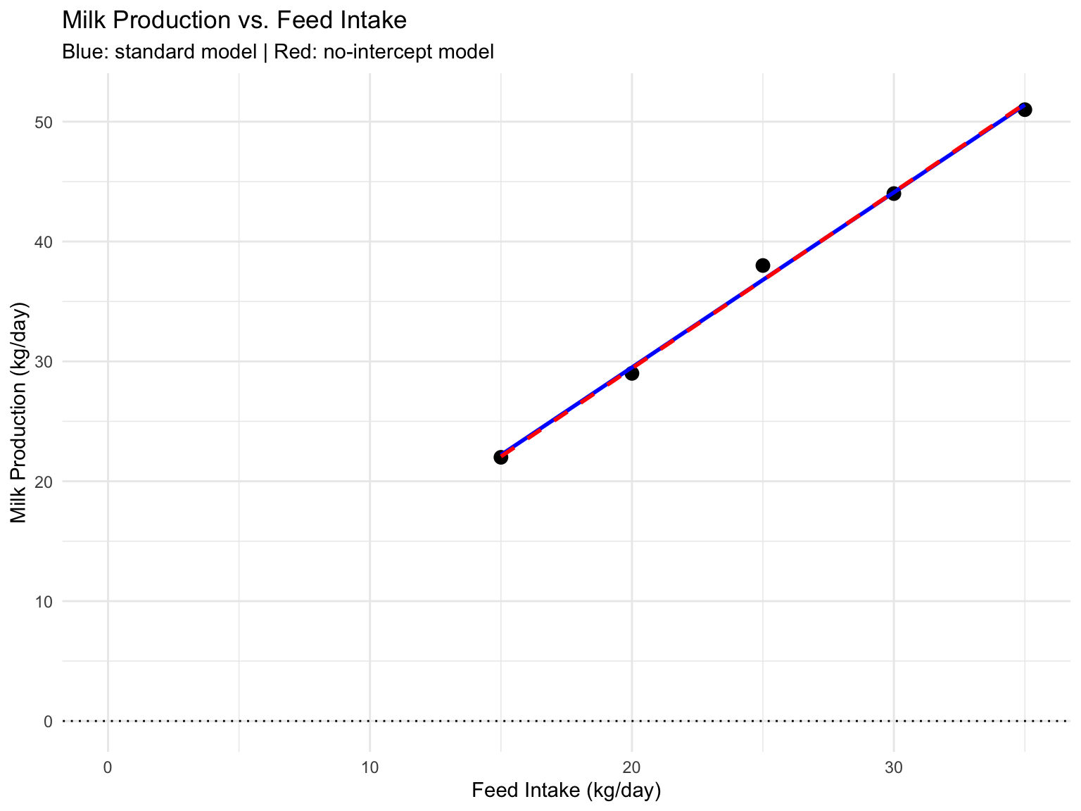
# Standard linear regression
fit_with_int <- lm(milk_production_kg ~ feed_intake_kg, data = milk_feed)
summary(fit_with_int)
Call:
lm(formula = milk_production_kg ~ feed_intake_kg, data = milk_feed)

Residuals:
   1    2    3    4    5
-0.2 -0.5  1.2 -0.1 -0.4

Coefficients:
               Estimate Std. Error t value Pr(>|t|)
(Intercept)     0.30000    1.30767   0.229    0.833
feed_intake_kg  1.46000    0.05033  29.007    9e-05 ***
---
Signif. codes:  0 '***' 0.001 '**' 0.01 '*' 0.05 '.' 0.1 ' ' 1

Residual standard error: 0.7958 on 3 degrees of freedom
Multiple R-squared:  0.9964,    Adjusted R-squared:  0.9953
F-statistic: 841.4 on 1 and 3 DF,  p-value: 8.997e-05
# Manual calculation
X_int <- cbind(1, milk_feed$feed_intake_kg)
y <- milk_feed$milk_production_kg
b_int <- solve(t(X_int) %*% X_int) %*% t(X_int) %*% y
cat("Manual estimates (with intercept):\n")Manual estimates (with intercept):print(b_int) [,1]
[1,] 0.30
[2,] 1.46Interpretation: Intercept is 1.71 kg/day. This suggests there’s some “baseline” milk production even before accounting for feed intake (biologically questionable).
# No-intercept regression
fit_no_int <- lm(milk_production_kg ~ feed_intake_kg - 1, data = milk_feed)
# or equivalently: lm(milk_production_kg ~ 0 + feed_intake_kg, data = milk_feed)
summary(fit_no_int)
Call:
lm(formula = milk_production_kg ~ feed_intake_kg - 1, data = milk_feed)

Residuals:
       1        2        3        4        5
-0.06667 -0.42222  1.22222 -0.13333 -0.48889

Coefficients:
               Estimate Std. Error t value Pr(>|t|)
feed_intake_kg  1.47111    0.01197   122.9 2.63e-08 ***
---
Signif. codes:  0 '***' 0.001 '**' 0.01 '*' 0.05 '.' 0.1 ' ' 1

Residual standard error: 0.6952 on 4 degrees of freedom
Multiple R-squared:  0.9997,    Adjusted R-squared:  0.9997
F-statistic: 1.511e+04 on 1 and 4 DF,  p-value: 2.626e-08
# Manual calculation
X_no_int <- matrix(milk_feed$feed_intake_kg, ncol = 1)
b_no_int <- solve(t(X_no_int) %*% X_no_int) %*% t(X_no_int) %*% y
cat("Manual estimate (no intercept):\n")Manual estimate (no intercept):print(b_no_int) [,1]
[1,] 1.471111# Verify formula
b1_formula <- sum(milk_feed$feed_intake_kg * milk_feed$milk_production_kg) /
sum(milk_feed$feed_intake_kg^2)
cat("Using formula: b₁ = Σ(xᵢyᵢ) / Σ(xᵢ²) =", b1_formula, "\n")Using formula: b₁ = Σ(xᵢyᵢ) / Σ(xᵢ²) = 1.471111 Interpretation: For each kg of feed intake, milk production increases by 1.46 kg/day. The line is forced through the origin.
# Residuals from both models
residuals_with <- residuals(fit_with_int)
residuals_no <- residuals(fit_no_int)

cat("Residuals WITH intercept:\n")
Residuals WITH intercept:print(round(residuals_with, 2)) 1 2 3 4 5
-0.2 -0.5 1.2 -0.1 -0.4 cat("Sum:", sum(residuals_with), "\n\n")Sum: 0 cat("Residuals NO intercept:\n")Residuals NO intercept:print(round(residuals_no, 2)) 1 2 3 4 5
-0.07 -0.42 1.22 -0.13 -0.49 cat("Sum:", sum(residuals_no), "(NOT zero!)\n")Sum: 0.1111111 (NOT zero!)With a standard intercept model, residuals always sum to zero: \(\sum e_i = 0\).
For no-intercept models, this is not guaranteed! Residuals can have a systematic bias.
# Sum of squared errors
SSE_with <- sum(residuals_with^2)
SSE_no <- sum(residuals_no^2)

cat("SSE (with intercept):", SSE_with, "\n")
SSE (with intercept): 1.9 cat("SSE (no intercept): ", SSE_no, "\n\n")SSE (no intercept): 1.933333 # R²
R2_with <- summary(fit_with_int)$r.squared
R2_no <- summary(fit_no_int)$r.squared
cat("R² (with intercept):", R2_with, "\n")R² (with intercept): 0.9964473 cat("R² (no intercept): ", R2_no, "\n")R² (no intercept): 0.9997354 For no-intercept models, \(R^2\) is calculated differently and can exceed 1.0 or be misleading. Do not compare \(R^2\) values between models with and without intercept!
The definition changes because SST (total sum of squares) changes:
We have weight gain and feed intake data for 40 broilers. Does it make sense to force through the origin?
# Load broiler gain-feed data
broiler_feed <- read.csv("data/broiler_gain_feed.csv")
head(broiler_feed, 10)| bird_id | feed_intake_kg | weight_gain_kg |
|---|---|---|
| 1 | 1.68 | 1.02 |
| 2 | 1.92 | 0.99 |
| 3 | 2.97 | 1.71 |
| 4 | 3.20 | 2.11 |
| 5 | 3.08 | 1.99 |
| 6 | 2.16 | 1.58 |
| 7 | 1.66 | 1.01 |
| 8 | 2.07 | 1.30 |
| 9 | 1.98 | 1.51 |
| 10 | 2.27 | 1.31 |
# Visualize with both models
ggplot(broiler_feed, aes(x = feed_intake_kg, y = weight_gain_kg)) +
  geom_point(alpha = 0.6) +
  geom_smooth(method = "lm", se = TRUE, color = "blue", fill = "lightblue") +
  geom_smooth(method = "lm", formula = y ~ x - 1, se = TRUE,
              color = "red", fill = "pink", linetype = "dashed") +
  expand_limits(x = 0, y = 0) +
  labs(title = "Broiler Weight Gain vs. Feed Intake (n=40)",
       subtitle = "Blue: standard model | Red: no-intercept model",
       x = "Feed Intake (kg)",
       y = "Weight Gain (kg)") +
  theme_minimal()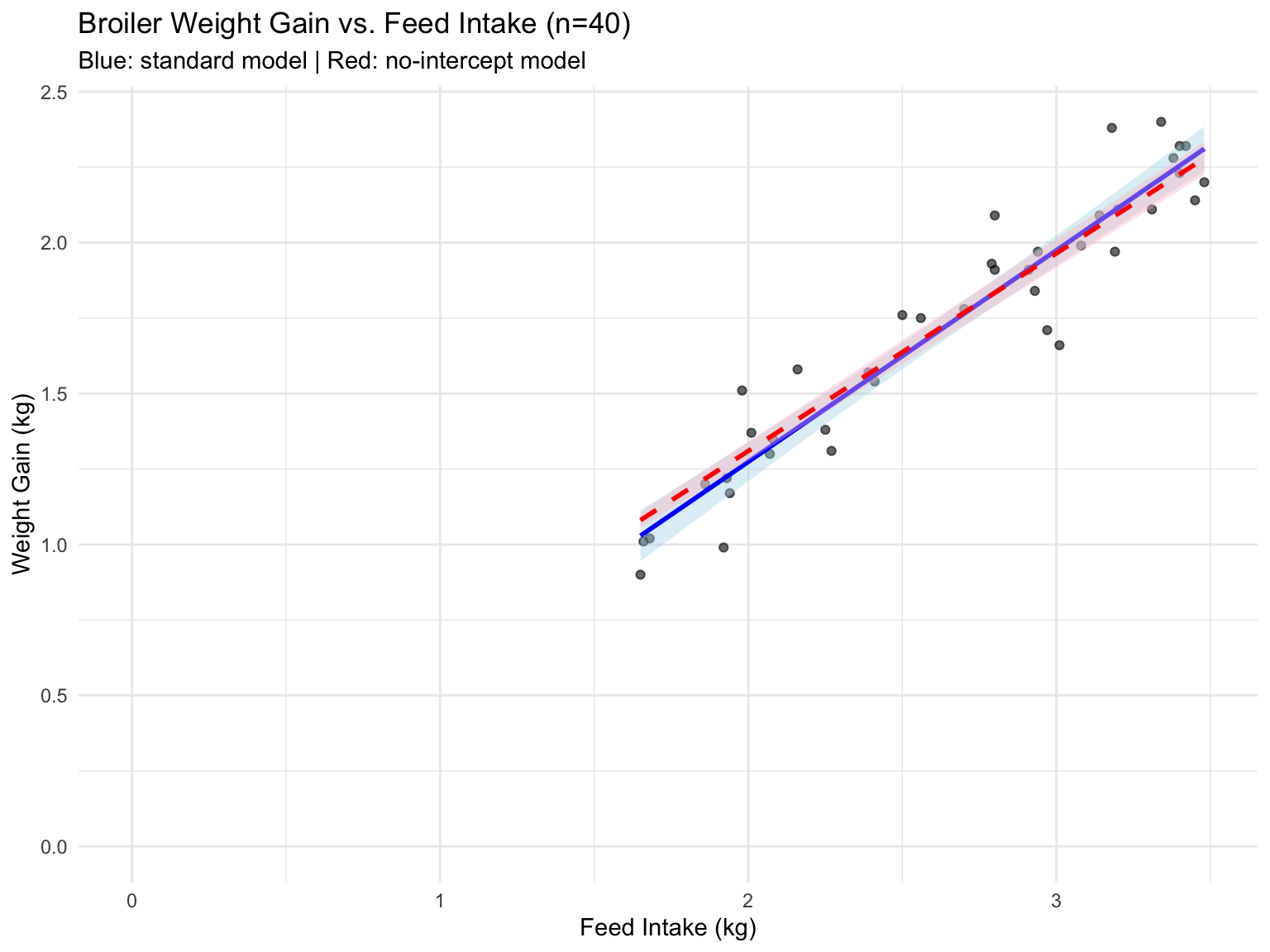
# Standard model
fit_broiler_std <- lm(weight_gain_kg ~ feed_intake_kg, data = broiler_feed)

# No-intercept model
fit_broiler_no <- lm(weight_gain_kg ~ feed_intake_kg - 1, data = broiler_feed)

# Compare coefficients
cat("Standard model:\n")
Standard model:print(coef(fit_broiler_std)) (Intercept) feed_intake_kg
-0.1270924 0.7005248 cat("\nNo-intercept model:\n")
No-intercept model:print(coef(fit_broiler_no))feed_intake_kg
0.6548412 # Is the intercept significantly different from zero?
cat("Standard model summary:\n")Standard model summary:print(summary(fit_broiler_std)$coefficients) Estimate Std. Error t value Pr(>|t|)
(Intercept) -0.1270924 0.09810467 -1.295478 2.029702e-01
feed_intake_kg 0.7005248 0.03610774 19.400958 2.593917e-21Interpretation: The intercept is -0.127 with SE = 0.098. The t-test (\(p\) = 0.203) shows the intercept is not significantly different from zero.
This suggests the no-intercept model might be reasonable here.
# Residual plots side by side
par(mfrow = c(1, 2))

# Standard model
plot(fitted(fit_broiler_std), residuals(fit_broiler_std),
     main = "Standard Model Residuals",
     xlab = "Fitted Values", ylab = "Residuals")
abline(h = 0, col = "red", lty = 2)

# No-intercept model
plot(fitted(fit_broiler_no), residuals(fit_broiler_no),
     main = "No-Intercept Model Residuals",
     xlab = "Fitted Values", ylab = "Residuals")
abline(h = 0, col = "red", lty = 2)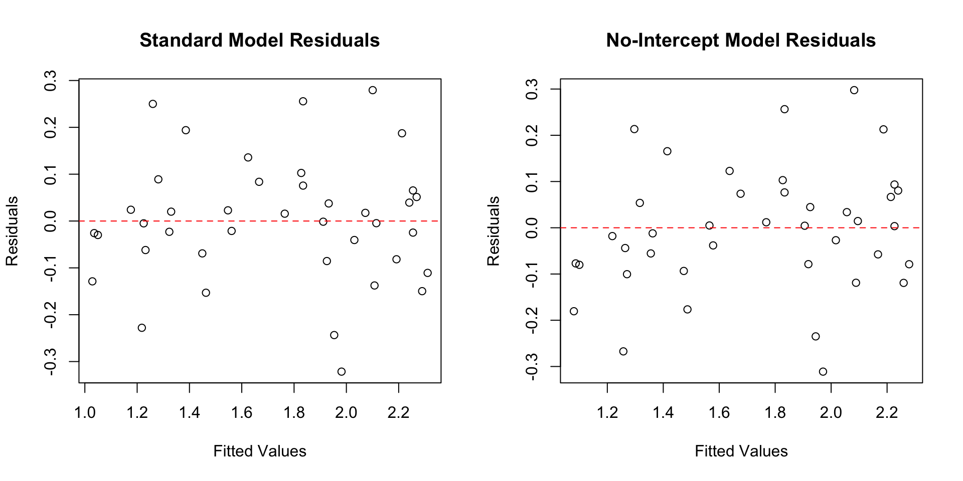
Both residual plots look reasonable—no strong patterns or heteroscedasticity.
Ask these questions:
General advice: Start with a standard model. Only remove the intercept if there’s strong justification.
When to consider:
Critical warnings:
R syntax:
lm(y ~ x - 1) or lm(y ~ 0 + x)Throughout this entire course, we’ve been fitting fixed effects models. The parameters \(\beta_0, \beta_1, \ldots, \beta_p\) are treated as fixed unknown constants that we estimate from data.
But in animal breeding and genetics, we often encounter random effects:
Random effects are parameters treated as random variables with a distribution. Instead of estimating a fixed value for each animal, we estimate:
This is the foundation of genetic evaluation, Estimated Progeny Differences (EPDs), and Genomic Selection.
In dairy cattle genetic evaluation:
Treating animal effects as fixed would:
Treating them as random:
This is why BLUP (Best Linear Unbiased Prediction) revolutionized animal breeding in the 1970s-1980s.
The general linear mixed model is:
\[ \boldsymbol{y} = \mathbf{X}\boldsymbol{\beta} + \mathbf{Z}\boldsymbol{u} + \boldsymbol{e} \]
where:
Key assumptions:
This is the first time in the course we introduce random effects notation:
Compare with what we’ve used all course:
In 1949, Charles Henderson derived the equations that simultaneously solve for fixed effects (\(\boldsymbol{\beta}\)) and predict random effects (\(\boldsymbol{u}\)).
For the general case:
\[ \begin{bmatrix} \mathbf{X}'\mathbf{R}^{-1}\mathbf{X} & \mathbf{X}'\mathbf{R}^{-1}\mathbf{Z} \\ \mathbf{Z}'\mathbf{R}^{-1}\mathbf{X} & \mathbf{Z}'\mathbf{R}^{-1}\mathbf{Z} + \mathbf{G}^{-1} \end{bmatrix} \begin{bmatrix} \hat{\boldsymbol{\beta}} \\ \hat{\boldsymbol{u}} \end{bmatrix} = \begin{bmatrix} \mathbf{X}'\mathbf{R}^{-1}\boldsymbol{y} \\ \mathbf{Z}'\mathbf{R}^{-1}\boldsymbol{y} \end{bmatrix} \]
This looks intimidating! But notice the similarity to our familiar normal equations:
\[ \mathbf{X}'\mathbf{X}\boldsymbol{b} = \mathbf{X}'\boldsymbol{y} \]
The MME are an augmented version that includes:
Simplified Case: When \(\mathbf{R} = \sigma^2\mathbf{I}\) and \(\mathbf{G} = \sigma_u^2\mathbf{I}\), the MME simplify to:
\[ \begin{bmatrix} \mathbf{X}'\mathbf{X} & \mathbf{X}'\mathbf{Z} \\ \mathbf{Z}'\mathbf{X} & \mathbf{Z}'\mathbf{Z} + \lambda\mathbf{I} \end{bmatrix} \begin{bmatrix} \hat{\boldsymbol{\beta}} \\ \hat{\boldsymbol{u}} \end{bmatrix} = \begin{bmatrix} \mathbf{X}'\boldsymbol{y} \\ \mathbf{Z}'\boldsymbol{y} \end{bmatrix} \]
where \(\lambda = \sigma^2 / \sigma_u^2\) is the variance ratio.
The variance ratio \(\lambda = \sigma^2 / \sigma_u^2\) controls the amount of shrinkage:
In animal breeding: \(\lambda\) relates to heritability!
\[ h^2 = \frac{\sigma_u^2}{\sigma_u^2 + \sigma^2} \]
High heritability → small \(\lambda\) → less shrinkage (genetics matters more than noise).
Solving the MME gives:
BLUP properties:
Everything you’ve learned applies to mixed models:
The only addition: An extra set of equations for random effects with a shrinkage penalty \(\mathbf{G}^{-1}\).
This course has given you the foundation to understand and implement mixed models!
Let’s fit a simple sire model where we compare treating sire as fixed vs. random.
Data: 5 sires with 3-5 daughters each (n=20 total cows).
# Load sire data
sire_data <- read.csv("data/simple_sire_model.csv")
sire_data| cow_id | sire | milk_yield |
|---|---|---|
| 1 | Sire1 | 84.1 |
| 2 | Sire1 | 83.2 |
| 3 | Sire1 | 85.7 |
| 4 | Sire1 | 81.5 |
| 5 | Sire1 | 90.3 |
| 6 | Sire2 | 76.2 |
| 7 | Sire2 | 73.2 |
| 8 | Sire2 | 77.3 |
| 9 | Sire2 | 75.8 |
| 10 | Sire3 | 89.6 |
| 11 | Sire3 | 81.1 |
| 12 | Sire3 | 87.1 |
| 13 | Sire4 | 82.5 |
| 14 | Sire4 | 86.6 |
| 15 | Sire4 | 81.7 |
| 16 | Sire4 | 82.0 |
| 17 | Sire5 | 87.3 |
| 18 | Sire5 | 79.6 |
| 19 | Sire5 | 85.8 |
| 20 | Sire5 | 76.8 |
# Summary by sire
sire_summary <- sire_data %>%
  group_by(sire) %>%
  summarise(
    n_daughters = n(),
    mean_yield = mean(milk_yield),
    sd_yield = sd(milk_yield)
  )
sire_summary| sire | n_daughters | mean_yield | sd_yield |
|---|---|---|---|
| Sire1 | 5 | 84.96000 | 3.349328 |
| Sire2 | 4 | 75.62500 | 1.736616 |
| Sire3 | 3 | 85.93333 | 4.368448 |
| Sire4 | 4 | 83.20000 | 2.290560 |
| Sire5 | 4 | 82.37500 | 4.992244 |
# Treat sire as fixed effect
fit_sire_fixed <- lm(milk_yield ~ sire, data = sire_data)
summary(fit_sire_fixed)
Call:
lm(formula = milk_yield ~ sire, data = sire_data)

Residuals:
    Min      1Q  Median      3Q     Max
-5.5750 -1.9263 -0.2625  2.1062  5.3400

Coefficients:
            Estimate Std. Error t value Pr(>|t|)
(Intercept)  84.9600     1.5603  54.451  < 2e-16 ***
sireSire2    -9.3350     2.3405  -3.989  0.00119 **
sireSire3     0.9733     2.5480   0.382  0.70782
sireSire4    -1.7600     2.3405  -0.752  0.46370
sireSire5    -2.5850     2.3405  -1.104  0.28679
---
Signif. codes:  0 '***' 0.001 '**' 0.01 '*' 0.05 '.' 0.1 ' ' 1

Residual standard error: 3.489 on 15 degrees of freedom
Multiple R-squared:  0.584, Adjusted R-squared:  0.4731
F-statistic: 5.265 on 4 and 15 DF,  p-value: 0.007477
# Get all sire estimates (using cell means model for clarity)
fit_sire_fixed_means <- lm(milk_yield ~ sire - 1, data = sire_data)
sire_fixed_estimates <- coef(fit_sire_fixed_means)
names(sire_fixed_estimates) <- levels(factor(sire_data$sire))
sire_fixed_estimates Sire1 Sire2 Sire3 Sire4 Sire5
84.96000 75.62500 85.93333 83.20000 82.37500 These are the daughter averages for each sire—no shrinkage, no borrowing of strength.
# Treat sire as random effect
library(lme4)
fit_sire_random <- lmer(milk_yield ~ 1 + (1|sire), data = sire_data)
summary(fit_sire_random)
Linear mixed model fit by REML ['lmerMod']
Formula: milk_yield ~ 1 + (1 | sire)
Data: sire_data
REML criterion at convergence: 111.1
Scaled residuals:
Min 1Q Median 3Q Max
-1.5986 -0.4914 -0.1783 0.6746 1.6445
Random effects:
Groups Name Variance Std.Dev.
sire (Intercept) 13.19 3.632
Residual 12.18 3.490
Number of obs: 20, groups: sire, 5
Fixed effects:
Estimate Std. Error t value
(Intercept) 82.397 1.806 45.63# Variance components
vc <- as.data.frame(VarCorr(fit_sire_random))
sigma_u <- vc$sdcor[1] # SD of sire effects
sigma_e <- vc$sdcor[2] # Residual SD
cat("Random effect SD (sire):", sigma_u, "\n")Random effect SD (sire): 3.632048 cat("Residual SD: ", sigma_e, "\n")Residual SD: 3.490063 cat("Variance ratio (λ): ", sigma_e^2 / sigma_u^2, "\n")Variance ratio (λ): 0.9233437 # BLUPs (Best Linear Unbiased Predictions)
sire_blups <- ranef(fit_sire_random)$sire[,1]
overall_mean <- fixef(fit_sire_random)
sire_random_predictions <- overall_mean + sire_blups
names(sire_random_predictions) <- rownames(ranef(fit_sire_random)$sire)
sire_random_predictions Sire1 Sire2 Sire3 Sire4 Sire5
84.56048 76.89505 85.10108 83.04941 82.37913 # Create comparison data frame
sire_comparison <- data.frame(
sire = names(sire_fixed_estimates),
n_daughters = sire_summary$n_daughters,
fixed_effect = as.numeric(sire_fixed_estimates),
random_effect = as.numeric(sire_random_predictions)
)
# Plot comparison
ggplot(sire_comparison, aes(x = sire)) +
geom_point(aes(y = fixed_effect, color = "Fixed Effects"), size = 3) +
geom_point(aes(y = random_effect, color = "Random Effects (BLUP)"), size = 3) +
geom_hline(yintercept = overall_mean, linetype = "dashed", color = "gray50") +
geom_text(aes(x = 1.5, y = overall_mean + 1.5,
label = paste("Overall mean =", round(overall_mean, 1))),
color = "gray30") +
scale_color_manual(values = c("Fixed Effects" = "blue",
"Random Effects (BLUP)" = "red")) +
labs(title = "Comparing Fixed Effects vs. Random Effects (BLUP)",
subtitle = "Notice shrinkage toward the population mean",
x = "Sire",
y = "Predicted Milk Yield (kg/day)",
color = "Method") +
theme_minimal() +
theme(legend.position = "bottom")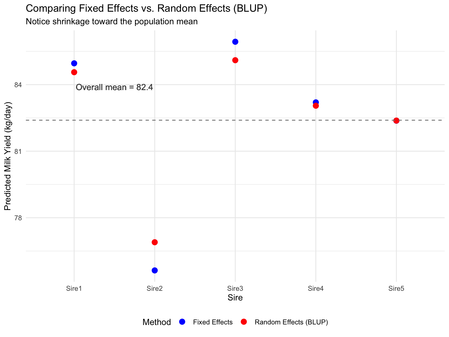
Notice how the BLUP estimates (red) are pulled toward the population mean compared to fixed effects (blue). This shrinkage is:
This is “borrowing strength”: Using information about the population distribution to improve predictions for individuals with sparse data.
This is exactly what happens in genetic evaluation: young bulls with few daughters get more shrinkage than proven bulls with many daughters.
# Quantify shrinkage
sire_comparison$shrinkage <- sire_comparison$fixed_effect - sire_comparison$random_effect
sire_comparison$shrinkage_pct <- (sire_comparison$shrinkage /
                                   (sire_comparison$fixed_effect - overall_mean)) * 100

cat("Shrinkage by sire:\n")
Shrinkage by sire:print(sire_comparison[, c("sire", "n_daughters", "shrinkage", "shrinkage_pct")]) sire n_daughters shrinkage shrinkage_pct
1 Sire1 5 0.399521335 15.58822
2 Sire2 4 -1.270053742 18.75440
3 Sire3 3 0.832255245 23.53461
4 Sire4 4 0.150592229 18.75440
5 Sire5 4 -0.004131589 18.75440Sires with fewer daughters experience more shrinkage—exactly as BLUP theory predicts!
Now let’s examine a more realistic scenario: 10 sires with varying numbers of daughters (3 to 25 per sire, n=100 total).
# Load dairy sire evaluation data
dairy_sire <- read.csv("data/dairy_sire_eval.csv")

# Summary by sire
dairy_summary <- dairy_sire %>%
  group_by(sire) %>%
  summarise(
    n_daughters = n(),
    mean_yield = mean(milk_yield),
    sd_yield = sd(milk_yield)
  ) %>%
  arrange(n_daughters)

dairy_summary| sire | n_daughters | mean_yield | sd_yield |
|---|---|---|---|
| Sire01 | 3 | 100.83333 | 4.244212 |
| Sire02 | 5 | 88.78000 | 8.473901 |
| Sire10 | 6 | 87.60000 | 4.616059 |
| Sire05 | 7 | 89.25714 | 4.340836 |
| Sire03 | 8 | 89.71250 | 4.508544 |
| Sire09 | 9 | 93.10000 | 6.859847 |
| Sire08 | 10 | 86.75000 | 4.714811 |
| Sire04 | 12 | 87.81667 | 7.718317 |
| Sire07 | 15 | 93.82667 | 4.175005 |
| Sire06 | 25 | 91.17600 | 6.043749 |
# Fixed effects model
fit_dairy_fixed <- lm(milk_yield ~ sire - 1, data = dairy_sire)
dairy_fixed_est <- coef(fit_dairy_fixed)

# Random effects model
fit_dairy_random <- lmer(milk_yield ~ 1 + (1|sire), data = dairy_sire)

# Extract estimates
dairy_overall_mean <- fixef(fit_dairy_random)
dairy_blups <- ranef(fit_dairy_random)$sire[,1]
dairy_random_pred <- dairy_overall_mean + dairy_blups
# Variance components
dairy_vc <- as.data.frame(VarCorr(fit_dairy_random))
cat("Sire variance (σ²ᵤ):", round(dairy_vc$vcov[1], 2), "\n")Sire variance (σ²ᵤ): 6.83 cat("Residual variance (σ²):", round(dairy_vc$vcov[2], 2), "\n")Residual variance (σ²): 34.48 cat("Variance ratio (λ):", round(dairy_vc$vcov[2] / dairy_vc$vcov[1], 2), "\n")Variance ratio (λ): 5.05 # Approximate heritability (sire model gives 1/4 h²)
h2_approx <- 4 * dairy_vc$vcov[1] / (dairy_vc$vcov[1] + dairy_vc$vcov[2])
cat("Approximate heritability:", round(h2_approx, 2), "\n")Approximate heritability: 0.66 # Comparison dataframe
dairy_comp <- data.frame(
sire = levels(factor(dairy_sire$sire)),
n_daughters = dairy_summary$n_daughters,
fixed = as.numeric(dairy_fixed_est),
blup = as.numeric(dairy_random_pred)
)
dairy_comp$shrinkage <- abs(dairy_comp$fixed - dairy_comp$blup)
# Plot: shrinkage vs. information
ggplot(dairy_comp, aes(x = n_daughters, y = shrinkage)) +
geom_point(size = 3, color = "darkred") +
geom_smooth(method = "loess", se = FALSE, color = "blue") +
labs(title = "Shrinkage Increases with Less Information",
subtitle = "Sires with fewer daughters experience more shrinkage toward population mean",
x = "Number of Daughters",
y = "Absolute Shrinkage (Fixed - BLUP)") +
theme_minimal()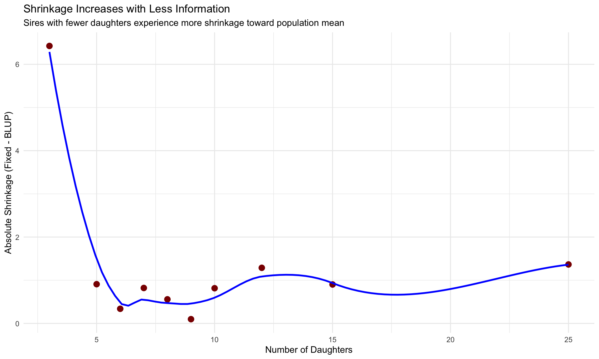
Perfect! As predicted by theory, shrinkage is inversely related to information: sires with fewer daughters get pulled more strongly toward the population mean.
# Plot fixed vs. BLUP estimates
dairy_comp_long <- dairy_comp %>%
  select(sire, n_daughters, fixed, blup) %>%
  pivot_longer(cols = c(fixed, blup), names_to = "method", values_to = "estimate")

ggplot(dairy_comp_long, aes(x = reorder(sire, n_daughters), y = estimate,
                             color = method, group = method)) +
  geom_point(size = 3) +
  geom_line(aes(group = sire), color = "gray70") +
  geom_hline(yintercept = dairy_overall_mean, linetype = "dashed", color = "black") +
  scale_color_manual(values = c("fixed" = "blue", "blup" = "red"),
                     labels = c("Fixed Effects", "BLUP")) +
  labs(title = "Fixed Effects vs. BLUP for 10 Dairy Sires",
       subtitle = "Ordered by number of daughters (left = few, right = many)",
       x = "Sire (ordered by information)",
       y = "Predicted Milk Yield (kg/day)",
       color = "Method") +
  theme_minimal() +
  theme(axis.text.x = element_text(angle = 45, hjust = 1),
        legend.position = "bottom")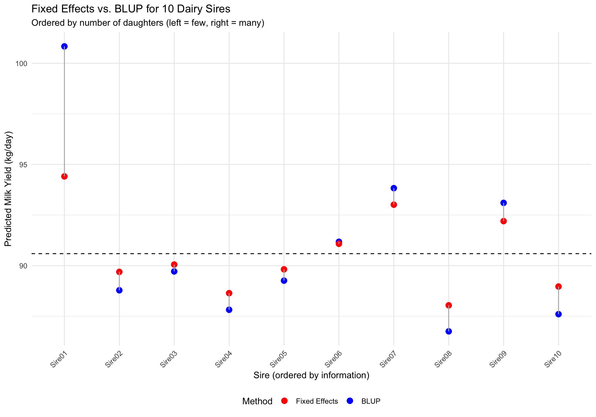
This demonstrates the power of BLUP for genetic evaluation:
In practice:
All build on the foundation you’ve learned in this course!
In livestock breeding, EPDs (Estimated Progeny Differences) are essentially BLUPs:
The EPDs you see in bull catalogs, sow selection indexes, and chicken breeding programs all come from mixed model equations—direct descendants of what we’ve studied this week!
Key concepts:
Why it matters:
What you’re ready for:
This course has prepared you with the matrix algebra, least squares theory, and linear model framework to understand and apply these advanced methods!
You have the following data on pig weight (kg) vs. age (weeks):
| Age (weeks) | Weight (kg) |
|---|---|
| 4 | 8 |
| 8 | 22 |
| 12 | 45 |
(a) Fit a quadratic model \(y = \beta_0 + \beta_1 x + \beta_2 x^2 + e\) by hand. Construct the \(\mathbf{X}\) matrix, compute \(\mathbf{X}'\mathbf{X}\) and \(\mathbf{X}'\boldsymbol{y}\), and solve for \(\boldsymbol{b}\).
(b) Predict the weight at age 16 weeks.
(c) Does the quadratic term (\(\beta_2\)) appear necessary based on the data pattern? Explain.
You have average daily gain (ADG, kg/day) data from 4 pens:
| Pen | ADG | Pen Size |
|---|---|---|
| 1 | 0.90 | 10 |
| 2 | 0.88 | 5 |
| 3 | 0.93 | 15 |
| 4 | 0.85 | 8 |
(a) Calculate the unweighted mean ADG (OLS estimate).
(b) Calculate the weighted mean ADG (WLS estimate) using weights \(w_i = n_i\) (pen size).
(c) Which estimate is more reliable and why?
Consider the no-intercept model \(y_i = \beta_1 x_i + e_i\).
(a) Prove that the residuals do not necessarily sum to zero: \(\sum e_i \neq 0\) in general.
(b) Show that the fitted values \(\hat{y}_i = b_1 x_i\) and observed values \(y_i\) do not necessarily have the same mean: \(\bar{\hat{y}} \neq \bar{y}\) in general.
(c) Explain why this property makes no-intercept models problematic if the true intercept is nonzero.
Using the lactation curve dataset (lactation_curve.csv):
(a) Fit linear, quadratic, and cubic models for milk yield vs. days in milk.
(b) Use anova() to test whether the quadratic term is needed. Report the F-statistic and p-value.
(c) Use anova() to test whether the cubic term (given quadratic is included) is needed.
(d) Compare adjusted R² for all three models. Which model would you recommend and why?
(e) Calculate VIF for the quadratic model with raw polynomials vs. orthogonal polynomials. Comment on collinearity.
Using the feed efficiency dataset (feed_efficiency_pens.csv):
(a) Fit an OLS model: fcr ~ diet (unweighted).
(b) Fit a WLS model: fcr ~ diet weighted by pen_size.
(c) Create a residual plot for the OLS model: plot |residuals| vs. pen size. Is there evidence of heteroscedasticity?
(d) Compare standard errors for diet effects between OLS and WLS. Which are smaller and why?
(e) Test the hypothesis \(H_0\): no diet effect using both models. Do your conclusions differ?
Using the broiler gain-feed dataset (broiler_gain_feed.csv):
(a) Fit a standard linear model: weight_gain_kg ~ feed_intake_kg.
(b) Test whether the intercept is significantly different from zero.
(c) Fit a no-intercept model: weight_gain_kg ~ feed_intake_kg - 1.
(d) Compare predictions at feed intake = 2.5 kg for both models.
(e) Plot both fitted lines on the same graph (extending to the origin). Which model seems more biologically plausible?
Consider a sheep breeding program with 20 rams, each with 5-15 offspring tested for weaning weight.
(a) Write out the mixed model equation for this scenario. Define all components (\(\boldsymbol{y}\), \(\mathbf{X}\), \(\boldsymbol{\beta}\), \(\mathbf{Z}\), \(\boldsymbol{u}\), \(\boldsymbol{e}\)).
(b) What are the fixed effects and what are the random effects?
(c) Explain conceptually why treating ram as a random effect is preferable to treating it as a fixed effect.
(d) If a ram has only 5 offspring while most have 15, how will the BLUP for this ram differ from the fixed effect estimate? Explain the shrinkage concept.
(e) If the estimated variance components are \(\sigma_u^2 = 4\) kg² and \(\sigma^2 = 16\) kg², calculate the variance ratio \(\lambda\) and approximate heritability \(h^2\).
This week, we explored four powerful extensions of the linear model framework:
Polynomial Regression enables us to model curved relationships common in animal science—growth curves, lactation curves, and response surfaces—while maintaining the linear model structure. Key takeaways: start with low degrees, use orthogonal polynomials to combat collinearity, and always prioritize biological plausibility over statistical fit.
Weighted Least Squares addresses heteroscedasticity by optimally weighting observations according to their precision. This is essential when working with grouped data, pen averages, or measurements with varying reliability. WLS provides more efficient estimates and valid inference when variances differ across observations.
Regression Through the Origin applies in special cases where theory dictates \(y=0\) when \(x=0\). While appealing, it requires careful justification and comes with important caveats about residual properties and \(R^2\) interpretation. Use sparingly!
Mixed Models bridge the gap between this course and advanced genetic evaluation methods. By introducing random effects, we can efficiently handle large numbers of effects, account for population structure, and preview BLUP—the foundation of modern animal breeding. Understanding the connection between the normal equations and Henderson’s MME shows how everything we’ve learned naturally extends to this powerful framework.
After completing this week, you can:
Next week, the Capstone Project integrates all concepts from Weeks 1-14. You’ll:
Everything comes together: matrix algebra, least squares theory, ANOVA, regression, diagnostics, and now these special topics. You’re ready!
Previous: Week 13: Special Topics I