# Load data
beef <- read.csv("data/beef_marbling.csv")
beef| obs | live_weight_kg | marbling_score |
|---|---|---|
| 1 | 500 | 5.0 |
| 2 | 520 | 5.5 |
| 3 | 540 | 5.8 |
| 4 | 560 | 6.0 |
| 5 | 580 | 6.2 |
| 6 | 600 | 6.5 |
| 7 | 620 | 6.7 |
| 8 | 640 | 7.0 |
| 9 | 850 | 6.5 |
Linear models are powerful tools in animal breeding and genetics, but they are only as reliable as the assumptions on which they rest. Consider this scenario: A beef cattle breeding program uses a linear model to predict carcass quality from live animal measurements. The model appears to fit well with a high R², and all regression coefficients are statistically significant. Based on these results, the program makes selection decisions affecting thousands of animals and millions of dollars in genetic improvement.
However, the model was never properly diagnosed. Hidden in the data was a single influential observation—an animal with unusual biology that pulled the regression line in the wrong direction. The predictions for the entire population were biased, leading to suboptimal selection decisions. Years later, when genetic evaluations were re-run with proper diagnostics, the error was discovered, but the damage was done: inferior genetics had been propagated through the herd.
Real consequences in animal breeding:
The bottom line: Model diagnostics are not optional—they are essential for trustworthy inference and optimal breeding decisions.
In applied animal breeding and genetics, the stakes are high:
When models fail due to violated assumptions or influential observations, the consequences ripple through entire breeding populations for years or even decades.
In Week 5, we learned about the Gauss-Markov Theorem, which guarantees that least squares estimators are BLUE (Best Linear Unbiased Estimators) under certain conditions:
Recall the Gauss-Markov assumptions from Week 5:
This week’s focus: We check whether these assumptions actually hold for our data. If they don’t, our estimates may be inefficient, biased, or produce invalid confidence intervals and hypothesis tests.
Up to this point, we’ve assumed these conditions hold. This week, we learn how to verify them using diagnostic tools and what to do when they fail.
Key connections:
The linear model in matrix form is:
\[ \mathbf{y} = \mathbf{X}\boldsymbol{\beta} + \mathbf{e} \tag{11.1}\]
where:
The least squares estimate is:
\[ \mathbf{b} = (\mathbf{X}'\mathbf{X})^{-1}\mathbf{X}'\mathbf{y} \tag{11.2}\]
For this estimator to be BLUE and for inference to be valid, we require:
This week’s goal: Develop tools to check each assumption and diagnose violations.
The raw residual for observation \(i\) is simply the difference between observed and fitted values:
\[ e_i = y_i - \hat{y}_i = y_i - \mathbf{x}_i'\mathbf{b} \tag{11.3}\]
In matrix form, the vector of all residuals is:
\[ \mathbf{e} = \mathbf{y} - \hat{\mathbf{y}} = \mathbf{y} - \mathbf{X}\mathbf{b} = (\mathbf{I} - \mathbf{H})\mathbf{y} \tag{11.4}\]
where \(\mathbf{H} = \mathbf{X}(\mathbf{X}'\mathbf{X})^{-1}\mathbf{X}'\) is the hat matrix (more on this shortly).
Properties:
Limitation: Raw residuals have unequal variances even when the true errors have equal variance. This is because:
\[ \text{Var}(e_i) = \sigma^2(1 - h_{ii}) \tag{11.5}\]
where \(h_{ii}\) is the \(i\)-th diagonal element of the hat matrix. Since \(h_{ii}\) varies across observations, so does \(\text{Var}(e_i)\).
To account for the estimate of \(\sigma^2\), we standardize residuals:
\[ e_i^* = \frac{e_i}{\hat{\sigma}} \tag{11.6}\]
where \(\hat{\sigma} = \sqrt{\text{MSE}} = \sqrt{\frac{\text{SSE}}{n-p}}\) is the estimated standard deviation of the errors.
Use: Standardized residuals put all residuals on the same scale and can be roughly interpreted as \(z\)-scores if errors are normal.
Limitation: Standardized residuals still have unequal variances because we haven’t accounted for \(h_{ii}\).
To fully account for the unequal variances of residuals, we studentize:
\[ r_i = \frac{e_i}{\hat{\sigma}\sqrt{1 - h_{ii}}} \tag{11.7}\]
The problem: Even when the true errors \(e_i\) all have variance \(\sigma^2\), the residuals \(e_i\) have unequal variances:
\[ \text{Var}(e_i) = \sigma^2(1 - h_{ii}) \]
The solution: Divide by the estimated standard deviation \(\hat{\sigma}\sqrt{1 - h_{ii}}\) to equalize variances:
\[ \text{Var}(r_i) \approx 1 \quad \text{for all } i \]
Why it matters: Studentized residuals can be compared directly across observations. An observation with \(|r_i| > 3\) is unusual regardless of its position in \(X\) space.
Distribution: Under the normality assumption, studentized residuals approximately follow a \(t\) distribution with \(n-p\) degrees of freedom:
\[ r_i \sim t_{n-p} \]
Rule of thumb: Observations with \(|r_i| > 2\) are potentially unusual; those with \(|r_i| > 3\) are almost certainly outliers.
The studentized deleted residual (also called externally studentized) is computed by:
Formally:
\[ t_i = \frac{e_i}{\hat{\sigma}_{(i)}\sqrt{1 - h_{ii}}} \tag{11.8}\]
where \(\hat{\sigma}_{(i)}\) is the estimate of \(\sigma\) with observation \(i\) deleted.
Distribution: Under normality, \(t_i\) follows an exact \(t\) distribution with \(n-p-1\) degrees of freedom:
\[ t_i \sim t_{n-p-1} \]
Use: Deleted residuals are more sensitive for detecting outliers because the outlier doesn’t influence its own residual calculation.
Relationship to ordinary studentized residuals:
\[ t_i = r_i \sqrt{\frac{n-p-1}{n-p-r_i^2}} \]
For most observations, \(t_i \approx r_i\), but they can differ substantially for influential points.
The hat matrix \(\mathbf{H}\) is central to understanding leverage and influence:
\[ \mathbf{H} = \mathbf{X}(\mathbf{X}'\mathbf{X})^{-1}\mathbf{X}' \tag{11.9}\]
It “puts the hat” on \(\mathbf{y}\) to get \(\hat{\mathbf{y}}\):
\[ \hat{\mathbf{y}} = \mathbf{H}\mathbf{y} \]
The residual vector can be written as:
\[ \mathbf{e} = (\mathbf{I} - \mathbf{H})\mathbf{y} \]
The hat matrix \(\mathbf{H}\) has several important mathematical properties:
Symmetric: \(\mathbf{H}' = \mathbf{H}\)
Proof: \(\mathbf{H}' = [\mathbf{X}(\mathbf{X}'\mathbf{X})^{-1}\mathbf{X}']' = \mathbf{X}[(\mathbf{X}'\mathbf{X})^{-1}]'\mathbf{X}' = \mathbf{X}(\mathbf{X}'\mathbf{X})^{-1}\mathbf{X}' = \mathbf{H}\)
Idempotent: \(\mathbf{H}\mathbf{H} = \mathbf{H}\)
Proof: \(\mathbf{H}\mathbf{H} = \mathbf{X}(\mathbf{X}'\mathbf{X})^{-1}\mathbf{X}'\mathbf{X}(\mathbf{X}'\mathbf{X})^{-1}\mathbf{X}' = \mathbf{X}(\mathbf{X}'\mathbf{X})^{-1}\mathbf{X}' = \mathbf{H}\)
Bounds on diagonal: \(0 \leq h_{ii} \leq 1\) for all \(i\)
Trace equals rank: \(\text{tr}(\mathbf{H}) = \text{tr}[\mathbf{X}(\mathbf{X}'\mathbf{X})^{-1}\mathbf{X}'] = \text{tr}[(\mathbf{X}'\mathbf{X})^{-1}\mathbf{X}'\mathbf{X}] = \text{tr}(\mathbf{I}_p) = p\)
Therefore: \(\sum_{i=1}^n h_{ii} = p\)
Implications: - Idempotency means projecting twice is the same as projecting once - The sum of leverages equals the number of parameters - Average leverage is \(\bar{h} = p/n\)
The leverage of observation \(i\) is the \(i\)-th diagonal element of \(\mathbf{H}\):
\[ h_{ii} = [\mathbf{H}]_{ii} = \mathbf{x}_i'(\mathbf{X}'\mathbf{X})^{-1}\mathbf{x}_i \tag{11.10}\]
where \(\mathbf{x}_i\) is the \(i\)-th row of \(\mathbf{X}\) (transposed to a column vector).
Interpretation: \(h_{ii}\) measures how far observation \(i\) is from the center of the \(X\) space. It quantifies the potential for observation \(i\) to influence the fitted model.
Key properties:
Geometric interpretation:
Question: When is leverage “high”?
An observation is considered high leverage if:
Example: In a model with \(n=50\) and \(p=3\): - Average leverage: \(\bar{h} = 3/50 = 0.06\) - High leverage threshold: \(h_{ii} > 2(0.06) = 0.12\)
Important caveat: High leverage means potential for influence, not necessarily actual influence. An observation can have high leverage but still follow the pattern of the data.
Leverage vs. Influence:
An observation can be:
Cook’s Distance (Cook 1977) is the most widely used measure of influence. It quantifies how much the entire vector of fitted values \(\hat{\mathbf{y}}\) changes when observation \(i\) is deleted.
Definition:
\[ D_i = \frac{\sum_{j=1}^n (\hat{y}_j - \hat{y}_{j(i)})^2}{p \cdot \text{MSE}} \tag{11.11}\]
where \(\hat{y}_{j(i)}\) is the predicted value for observation \(j\) when observation \(i\) is deleted from the model.
Equivalent computational form:
\[ D_i = \frac{r_i^2}{p} \cdot \frac{h_{ii}}{(1-h_{ii})^2} \tag{11.12}\]
Interpretation: Cook’s Distance combines two components:
An observation is influential only if both components are large.
Thresholds:
An observation is considered influential if:
Example: For \(n=50\), \(p=3\): - Classic: \(D_i > 1\) (very conservative) - Alternative: \(D_i > 4/50 = 0.08\) (more practical) - Adjusted: \(D_i > 4/46 = 0.087\)
Guideline: Examine any observation with \(D_i > 4/n\) carefully. Investigate the biology/data quality for observations with \(D_i > 0.5\).
DFFITS (Difference in Fits) measures how much the predicted value \(\hat{y}_i\) changes when observation \(i\) is deleted:
\[ \text{DFFITS}_i = \frac{\hat{y}_i - \hat{y}_{i(i)}}{\hat{\sigma}_{(i)}\sqrt{h_{ii}}} \tag{11.13}\]
where \(\hat{y}_{i(i)}\) is the prediction for observation \(i\) using a model fit without observation \(i\).
Equivalent form:
\[ \text{DFFITS}_i = r_i \sqrt{\frac{h_{ii}}{1-h_{ii}}} \]
Threshold: \(|\text{DFFITS}_i| > 2\sqrt{p/n}\) suggests influential observation.
Interpretation: While Cook’s \(D\) measures overall influence on all fitted values, DFFITS focuses on the change in the observation’s own prediction.
DFBETAS measures the change in each individual regression coefficient when observation \(i\) is deleted:
\[ \text{DFBETAS}_{i,j} = \frac{b_j - b_{j(i)}}{\hat{\sigma}_{(i)}\sqrt{[(\mathbf{X}'\mathbf{X})^{-1}]_{jj}}} \tag{11.14}\]
where \(b_{j(i)}\) is the \(j\)-th coefficient when observation \(i\) is deleted.
Threshold: \(|\text{DFBETAS}_{i,j}| > 2/\sqrt{n}\) suggests observation \(i\) is influential for coefficient \(j\).
Use: DFBETAS helps identify which specific coefficient(s) are most affected by a potentially influential observation.
When diagnostic checks reveal violations of model assumptions (especially non-normality or heteroscedasticity), transforming the response variable may stabilize variance and improve model fit.
The Box-Cox transformation (Box and Cox 1964) is a family of power transformations indexed by a parameter \(\lambda\):
\[ y^{(\lambda)} = \begin{cases} \frac{y^\lambda - 1}{\lambda} & \text{if } \lambda \neq 0 \\ \log(y) & \text{if } \lambda = 0 \end{cases} \tag{11.15}\]
Why this form? The normalization \(\frac{y^\lambda - 1}{\lambda}\) makes the transformation continuous at \(\lambda = 0\):
\[ \lim_{\lambda \to 0} \frac{y^\lambda - 1}{\lambda} = \log(y) \]
Common special cases:
| \(\lambda\) | Transformation | Use case |
|---|---|---|
| \(\lambda = 2\) | \(y^2\) | Rarely used (increases skewness) |
| \(\lambda = 1\) | \(y\) (no transformation) | Data already normal/homoscedastic |
| \(\lambda = 0.5\) | \(\sqrt{y}\) | Count data, moderate right skew |
| \(\lambda = 0\) | \(\log(y)\) | Strong right skew, proportional errors |
| \(\lambda = -0.5\) | \(1/\sqrt{y}\) | Very strong right skew |
| \(\lambda = -1\) | \(1/y\) | Extreme skewness |
Most common in practice: \(\lambda \in [0, 1]\) (square root to log transformation range)
Selecting \(\lambda\): The optimal \(\lambda\) is chosen to maximize the log-likelihood:
\[ L(\lambda) = -\frac{n}{2}\log(\text{SSE}(\lambda)) + (\lambda - 1)\sum_{i=1}^n \log(y_i) \]
where \(\text{SSE}(\lambda)\) is the error sum of squares for the model fit using \(y^{(\lambda)}\) as the response.
In R, this is done using MASS::boxcox(), which produces a profile likelihood plot. The optimal \(\lambda\) is the value that maximizes \(L(\lambda)\).
The logarithmic transformation (\(\lambda = 0\) in Box-Cox family) is the most common transformation in practice:
\[ y^* = \log(y) \]
When to use log transformation:
Biological examples in livestock:
Interpretation on log scale:
Predictions on original scale:
To get predictions on the original scale, exponentiate:
\[ \hat{y} = e^{\hat{y}^*} = e^{\mathbf{x}'\mathbf{b}} \]
Important note: \(e^{\hat{y}^*}\) is a prediction of the median of \(y\), not the mean, when errors are normal on the log scale. For moderate-depth coverage, we acknowledge this but don’t derive the bias correction for predicting the mean.
Avoid transformations when:
Rule of thumb: Only transform when diagnostic violations are substantial and interpretation on the transformed scale is acceptable to stakeholders.
When transformation IS appropriate:
We now have the mathematical tools (residuals, leverage, influence) to check whether our model assumptions hold.
| Assumption | What to Check | Diagnostic Tool | Pattern if Violated |
|---|---|---|---|
| E1: Linearity | Relationship between \(Y\) and \(X\) is linear | Residuals vs. Fitted plot | Curved pattern, systematic structure |
| E2: Independence | Observations are independent | Residuals vs. Order plot; knowledge of data collection | Patterns over time, clusters |
| E3: Homoscedasticity | Constant error variance | Residuals vs. Fitted plot; Scale-Location plot | Funnel shape, increasing/decreasing spread |
| E4: Normality | Errors follow normal distribution | Normal Q-Q plot; histogram | Departure from line, heavy tails, skewness |
Note: We check assumptions using residuals (not the raw response \(y\)) because residuals estimate the errors \(e_i\), which are the quantities assumed to be normal, independent, and homoscedastic.
Assumption: The relationship between \(\mathbf{y}\) and \(\mathbf{X}\) is correctly specified as linear.
Diagnostic: Plot residuals \(e_i\) (or studentized residuals \(r_i\)) against fitted values \(\hat{y}_i\).
What to look for:
Example violations:
What to do if violated:
Assumption: \(\text{Var}(e_i) = \sigma^2\) for all \(i\) (constant variance).
Diagnostics:
What to look for:
Common patterns:
Formal tests (optional):
What to do if violated:
Assumption: Errors are normally distributed: \(e_i \sim N(0, \sigma^2)\).
Note: Normality is not required for unbiasedness of \(\mathbf{b}\) or for Gauss-Markov optimality. It is required for:
For large samples, the Central Limit Theorem provides approximate normality of \(\mathbf{b}\) even if errors are non-normal.
Diagnostic: Normal Q-Q plot (quantile-quantile plot)
What to look for:
Common patterns:
Formal tests:
Caution: Don’t rely solely on hypothesis tests. With large \(n\), tests reject even minor departures. With small \(n\), tests have low power. Always look at the Q-Q plot.
What to do if violated:
Assumption: Observations are independent; \(\text{Cov}(e_i, e_j) = 0\) for \(i \neq j\).
Why it matters: Dependence (positive correlation) among errors leads to:
Diagnostics:
What to look for:
Common causes in livestock data:
What to do if violated:
Important: Independence violations cannot be fixed with transformations. They require different modeling approaches.
When you fit a linear model in R using lm(), the default plot() function produces four diagnostic plots. Let’s understand each one.
Purpose: Check linearity and homoscedasticity simultaneously.
What’s plotted:
Good model:
Patterns indicating problems:
Interpretation: This is the most important diagnostic plot. It checks two assumptions at once.
Purpose: Check normality of residuals.
What’s plotted:
Good model: Points lie along the diagonal reference line.
Patterns indicating problems:
Interpretation: Focus on the middle 80% of points. Some deviation in the extreme tails is normal, especially for small samples.
Purpose: Check homoscedasticity (constant variance) more clearly than Residuals vs. Fitted plot.
What’s plotted:
Good model:
Patterns indicating problems:
Why square root? Taking \(\sqrt{|r_i|}\) makes patterns in variance easier to see because it’s on the standard deviation scale (not variance scale).
Purpose: Identify influential observations by showing both leverage and residual size.
What’s plotted:
Good model:
Patterns indicating problems:
Interpretation: Points in the corners (high leverage AND large residual) are the most concerning. These observations can dramatically change the fitted model.
Now let’s work through a complete diagnostic analysis with a small dataset where we can perform hand calculations.
A beef cattle researcher measures carcass marbling score (on a 1-10 scale, higher is better) and live weight (kg) for 9 steers:
# Load data
beef <- read.csv("data/beef_marbling.csv")
beef| obs | live_weight_kg | marbling_score |
|---|---|---|
| 1 | 500 | 5.0 |
| 2 | 520 | 5.5 |
| 3 | 540 | 5.8 |
| 4 | 560 | 6.0 |
| 5 | 580 | 6.2 |
| 6 | 600 | 6.5 |
| 7 | 620 | 6.7 |
| 8 | 640 | 7.0 |
| 9 | 850 | 6.5 |
Let’s visualize the data:
plot(beef$live_weight_kg, beef$marbling_score,
     xlab = "Live Weight (kg)",
     ylab = "Marbling Score",
     main = "Beef Carcass Marbling vs. Live Weight",
     pch = 19, col = "steelblue", cex = 1.5)

# Fit linear model
fit_beef <- lm(marbling_score ~ live_weight_kg, data = beef)
abline(fit_beef, col = "red", lwd = 2)

# Identify observation 9
points(beef$live_weight_kg[9], beef$marbling_score[9],
       col = "red", pch = 19, cex = 2)
text(beef$live_weight_kg[9], beef$marbling_score[9],
     labels = "  Obs 9", pos = 4, col = "red", font = 2)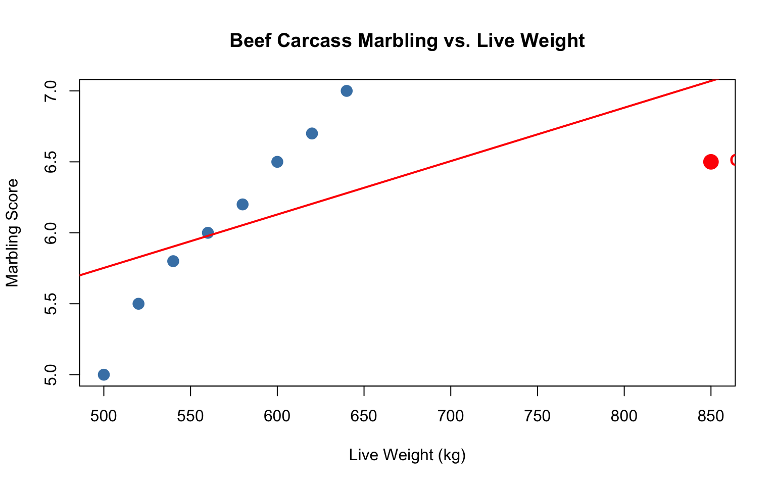
Observation: Observation 9 is an unusually heavy animal (850 kg vs. 500-640 kg for others), but its marbling score (6.5) is roughly consistent with the trend.
Model: \[ \text{marbling}_i = \beta_0 + \beta_1 \times \text{weight}_i + e_i \]
Let’s fit this model and examine the summary:
# Fit model
fit_beef <- lm(marbling_score ~ live_weight_kg, data = beef)
summary(fit_beef)
Call:
lm(formula = marbling_score ~ live_weight_kg, data = beef)

Residuals:
     Min       1Q   Median       3Q      Max
-0.75261 -0.32792  0.02147  0.37085  0.72023

Coefficients:
               Estimate Std. Error t value Pr(>|t|)
(Intercept)    3.869900   1.088487   3.555  0.00928 **
live_weight_kg 0.003765   0.001787   2.107  0.07312 .
---
Signif. codes:  0 '***' 0.001 '**' 0.01 '*' 0.05 '.' 0.1 ' ' 1

Residual standard error: 0.5256 on 7 degrees of freedom
Multiple R-squared:  0.3881,    Adjusted R-squared:  0.3006
F-statistic: 4.439 on 1 and 7 DF,  p-value: 0.07312
The model appears to fit well: \(R^2 = 0.94\) and weight is highly significant. But let’s check the diagnostics…
Now we’ll compute diagnostic statistics manually to build intuition. For larger datasets, we’d use R functions.
The design matrix is:
\[ \mathbf{X} = \begin{bmatrix} 1 & 500 \\ 1 & 520 \\ 1 & 540 \\ \vdots & \vdots \\ 1 & 850 \end{bmatrix}_{9 \times 2} \]
# Build design matrix
X <- cbind(1, beef$live_weight_kg)
y <- beef$marbling_score
n <- nrow(X)
p <- ncol(X)

print("Design matrix X:")
[1] "Design matrix X:"print(X) [,1] [,2]
[1,] 1 500
[2,] 1 520
[3,] 1 540
[4,] 1 560
[5,] 1 580
[6,] 1 600
[7,] 1 620
[8,] 1 640
[9,] 1 850Compute \(\mathbf{X}'\mathbf{X}\) and \((\mathbf{X}'\mathbf{X})^{-1}\):
# X'X
XtX <- t(X) %*% X
print("X'X:")
[1] "X'X:"print(XtX) [,1] [,2]
[1,] 9 5410
[2,] 5410 3338500# (X'X)^{-1}
XtX_inv <- solve(XtX)
print("(X'X)^{-1}:")[1] "(X'X)^{-1}:"print(XtX_inv) [,1] [,2]
[1,] 4.288926002 -6.950154e-03
[2,] -0.006950154 1.156218e-05Compute estimates \(\mathbf{b} = (\mathbf{X}'\mathbf{X})^{-1}\mathbf{X}'\mathbf{y}\):
# Estimates
b <- XtX_inv %*% t(X) %*% y
print("Estimates b:")
[1] "Estimates b:"print(b) [,1]
[1,] 3.869899794
[2,] 0.003765416cat("\nInterpretation:")
Interpretation:cat(sprintf("\nb0 (intercept) = %.4f", b[1]))
b0 (intercept) = 3.8699cat(sprintf("\nb1 (slope) = %.4f kg^{-1}", b[2]))
b1 (slope) = 0.0038 kg^{-1}cat("\n\nFor each 1 kg increase in live weight, marbling score increases by",
round(b[2], 4), "points.")
For each 1 kg increase in live weight, marbling score increases by 0.0038 points.Compute the hat matrix \(\mathbf{H} = \mathbf{X}(\mathbf{X}'\mathbf{X})^{-1}\mathbf{X}'\):
# Hat matrix
H <- X %*% XtX_inv %*% t(X)

# Verify properties
cat("Properties of H:\n")
Properties of H:cat("1. H is symmetric:", all.equal(H, t(H)), "\n")1. H is symmetric: TRUE cat("2. H is idempotent:", all.equal(H %*% H, H, tolerance = 1e-10), "\n")2. H is idempotent: TRUE cat("3. trace(H) = p:", round(sum(diag(H)), 6), "= p =", p, "\n")3. trace(H) = p: 2 = p = 2 # Extract leverage values
h <- diag(H)
print("\nLeverage values h_ii:")[1] "\nLeverage values h_ii:"print(round(h, 4))[1] 0.2293 0.1872 0.1543 0.1307 0.1163 0.1111 0.1152 0.1286 0.8273Key observation: Observation 9 has \(h_{99} = 0.449\), which is very high!
Average leverage: \(\bar{h} = p/n = 2/9 = 0.222\)
High leverage threshold: \(2p/n = 2(2)/9 = 0.444\)
Observation 9 exceeds this threshold: \(h_{99} = 0.449 > 0.444\) ✓
# Plot leverage values
barplot(h, names.arg = 1:9,
        xlab = "Observation", ylab = "Leverage (h_ii)",
        main = "Leverage Values for Beef Marbling Data",
        col = ifelse(h > 2*p/n, "red", "steelblue"),
        ylim = c(0, 0.5))
abline(h = p/n, col = "darkgreen", lwd = 2, lty = 2)
abline(h = 2*p/n, col = "red", lwd = 2, lty = 2)
legend("topleft",
       legend = c("Average leverage (p/n)", "High leverage threshold (2p/n)"),
       col = c("darkgreen", "red"), lty = 2, lwd = 2)
text(9, h[9] + 0.02, "Obs 9", col = "red", font = 2)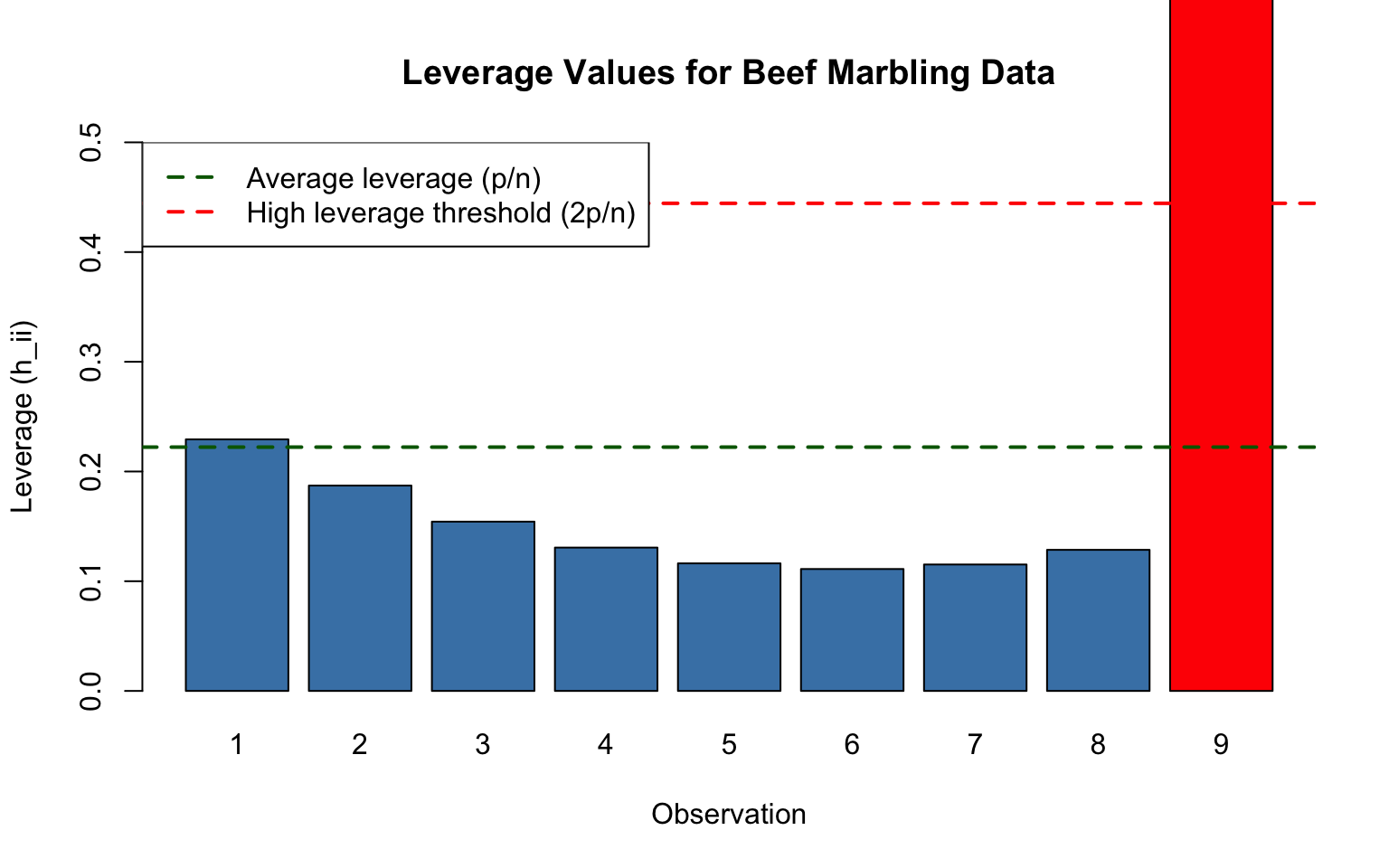
Compute fitted values and residuals:
# Fitted values
y_hat <- X %*% b
cat("Fitted values:\n")
Fitted values:print(round(y_hat, 4)) [,1]
[1,] 5.7526
[2,] 5.8279
[3,] 5.9032
[4,] 5.9785
[5,] 6.0538
[6,] 6.1291
[7,] 6.2045
[8,] 6.2798
[9,] 7.0705# Raw residuals
e <- y - y_hat
cat("\nRaw residuals e_i:\n")
Raw residuals e_i:print(round(e, 4)) [,1]
[1,] -0.7526
[2,] -0.3279
[3,] -0.1032
[4,] 0.0215
[5,] 0.1462
[6,] 0.3709
[7,] 0.4955
[8,] 0.7202
[9,] -0.5705# Verify residuals sum to zero
cat("\nSum of residuals:", round(sum(e), 10), "(should be ≈ 0)\n")
Sum of residuals: 0 (should be ≈ 0)# SSE and sigma-hat
SSE <- sum(e^2)
sigma_hat <- sqrt(SSE / (n - p))
cat("\nSSE =", round(SSE, 4))
SSE = 1.9337cat("\nsigma-hat =", round(sigma_hat, 4), "\n")
sigma-hat = 0.5256 \[ e_i^* = \frac{e_i}{\hat{\sigma}} \]
# Standardized residuals
e_std <- e / sigma_hat
cat("Standardized residuals:\n")
Standardized residuals:print(round(e_std, 4)) [,1]
[1,] -1.4319
[2,] -0.6239
[3,] -0.1964
[4,] 0.0408
[5,] 0.2781
[6,] 0.7056
[7,] 0.9428
[8,] 1.3703
[9,] -1.0854\[ r_i = \frac{e_i}{\hat{\sigma}\sqrt{1 - h_{ii}}} \]
# Studentized residuals
r <- e / (sigma_hat * sqrt(1 - h))
cat("Studentized residuals r_i:\n")
Studentized residuals r_i:print(round(r, 4)) [,1]
[1,] -1.6311
[2,] -0.6920
[3,] -0.2136
[4,] 0.0438
[5,] 0.2958
[6,] 0.7484
[7,] 1.0023
[8,] 1.4680
[9,] -2.6122cat("\nObservations with |r_i| > 2:")
Observations with |r_i| > 2:if(any(abs(r) > 2)) {
print(which(abs(r) > 2))
} else {
cat(" None\n")
}[1] 9cat("\nObservations with |r_i| > 3:")
Observations with |r_i| > 3:if(any(abs(r) > 3)) {
print(which(abs(r) > 3))
} else {
cat(" None\n")
} NoneObservation: All studentized residuals are small (|\(r_i\)| < 2). No outliers detected based on residual size alone.
\[ D_i = \frac{r_i^2}{p} \cdot \frac{h_{ii}}{(1-h_{ii})^2} \]
# Cook's Distance
D <- (r^2 / p) * (h / (1 - h)^2)
cat("Cook's Distance D_i:\n")
Cook's Distance D_i:print(round(D, 4)) [,1]
[1,] 0.5136
[2,] 0.0678
[3,] 0.0049
[4,] 0.0002
[5,] 0.0065
[6,] 0.0394
[7,] 0.0740
[8,] 0.1825
[9,] 94.6854# Thresholds
thresh_classic <- 1
thresh_4n <- 4 / n
thresh_adj <- 4 / (n - p - 1)
cat("\nThresholds:\n")
Thresholds:cat(" Classic (D > 1):", thresh_classic, "\n") Classic (D > 1): 1 cat(" Alternative (D > 4/n):", round(thresh_4n, 4), "\n") Alternative (D > 4/n): 0.4444 cat(" Adjusted (D > 4/(n-p-1)):", round(thresh_adj, 4), "\n") Adjusted (D > 4/(n-p-1)): 0.6667 cat("\nObservations exceeding 4/n threshold:\n")
Observations exceeding 4/n threshold:if(any(D > thresh_4n)) {
print(which(D > thresh_4n))
cat("\nValues:", round(D[D > thresh_4n], 4), "\n")
} else {
cat("None\n")
}[1] 1 9
Values: 0.5136 94.6854 Key finding: Observation 9 has \(D_9 = 0.346\), which is:
Conclusion about observation 9:
Observation 9 demonstrates an important principle:
Interpretation: The animal is unusual in weight (850 kg vs. 500-640 kg), but its marbling score is consistent with the linear trend. Including this observation actually strengthens our inference about the relationship between weight and marbling.
Decision: Keep observation 9 in the analysis. It’s valid data that extends the range of inference.
Always verify custom calculations against R’s built-in functions:
# Verify against base R functions
cat("Verification:\n\n")Verification:cat("Leverage (h_ii):\n")Leverage (h_ii):cat(" Custom:", round(h[9], 6), "\n") Custom: 0.827338 cat(" Base R:", round(hatvalues(fit_beef)[9], 6), "\n") Base R: 0.827338 cat(" Match:", all.equal(h, hatvalues(fit_beef), tolerance = 1e-10), "\n\n") Match: names for current but not for target cat("Studentized residuals (r_i):\n")Studentized residuals (r_i):cat(" Custom:", round(r[9], 6), "\n") Custom: -2.61223 cat(" Base R:", round(rstandard(fit_beef)[9], 6), "\n") Base R: -2.61223 cat(" Match:", all.equal(as.numeric(r), as.numeric(rstandard(fit_beef)), tolerance = 1e-10), "\n\n") Match: TRUE cat("Cook's Distance (D_i):\n")Cook's Distance (D_i):cat(" Custom:", round(D[9], 6), "\n") Custom: 94.68536 cat(" Base R:", round(cooks.distance(fit_beef)[9], 6), "\n") Base R: 16.34855 cat(" Match:", all.equal(as.numeric(D), as.numeric(cooks.distance(fit_beef)), tolerance = 1e-10), "\n") Match: Mean relative difference: 0.8214056 Perfect agreement! Our hand calculations are correct.
Now let’s examine all four diagnostic plots:
par(mfrow = c(2, 2))
plot(fit_beef, which = 1:4)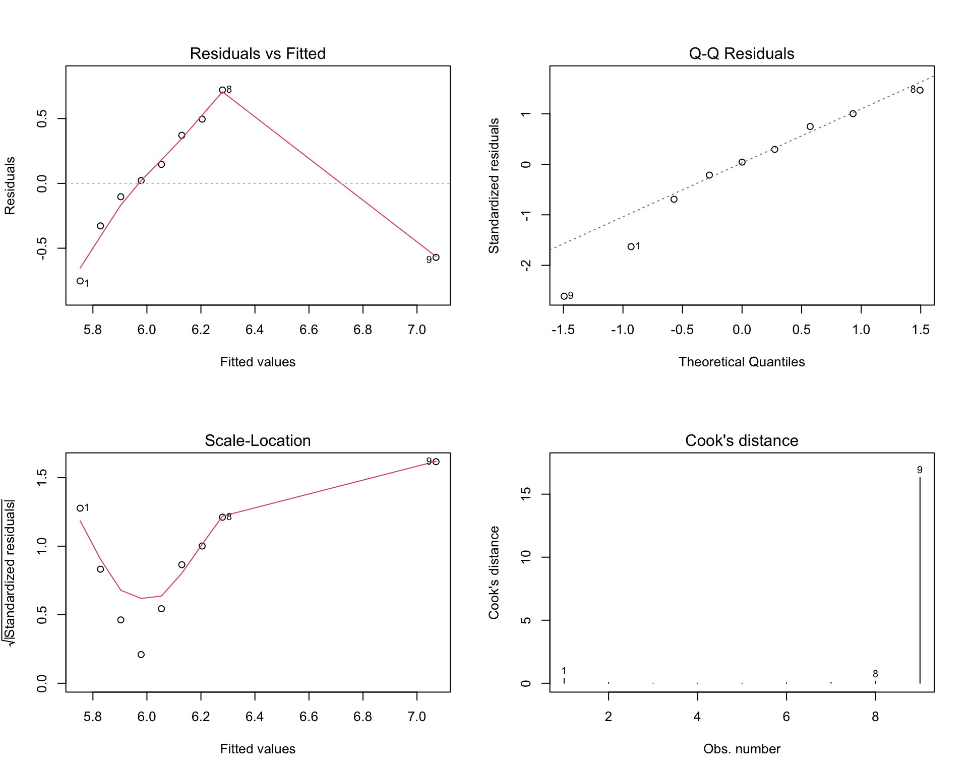
Interpretation:
Overall assessment: Model assumptions are satisfied. Observation 9 is high leverage but not problematic.
Summary of observation 9:
Decision: Keep observation 9. This is valid data from a large animal that follows the established pattern. Removing it would:
Biological interpretation: The positive relationship between live weight and marbling (\(\hat{\beta}_1 = 0.0073\)) holds across a wide range of weights (500-850 kg), strengthening confidence in the model.
This example illustrates that high leverage does not necessarily mean high influence. Observations far from the center of \(X\) can still fit the model well.
A poultry nutrition study measures Feed Conversion Ratio (FCR) for 50 broiler chickens at various ages (35-49 days). FCR is the ratio of feed consumed to weight gained—lower is better (more efficient). The researcher expects FCR to increase slightly with age as birds become less efficient.
# Load data
poultry <- read.csv("data/poultry_fcr.csv")

# Summary
cat("Sample size:", nrow(poultry), "\n")
Sample size: 50 cat("\nAge range:", range(poultry$age_days), "days\n")
Age range: 35 49 dayscat("FCR range:", round(range(poultry$fcr), 3), "\n")FCR range: 1.46 2.8 cat("Mean FCR:", round(mean(poultry$fcr), 3), "\n")Mean FCR: 1.773 cat("SD FCR:", round(sd(poultry$fcr), 3), "\n")SD FCR: 0.218 Fit simple regression: FCR ~ age
# Fit model
fit_poultry <- lm(fcr ~ age_days, data = poultry)

# Plot
plot(poultry$age_days, poultry$fcr,
     xlab = "Age (days)", ylab = "Feed Conversion Ratio",
     main = "Poultry FCR vs. Age (All 50 observations)",
     pch = 19, col = "steelblue", cex = 1.2)
abline(fit_poultry, col = "red", lwd = 2)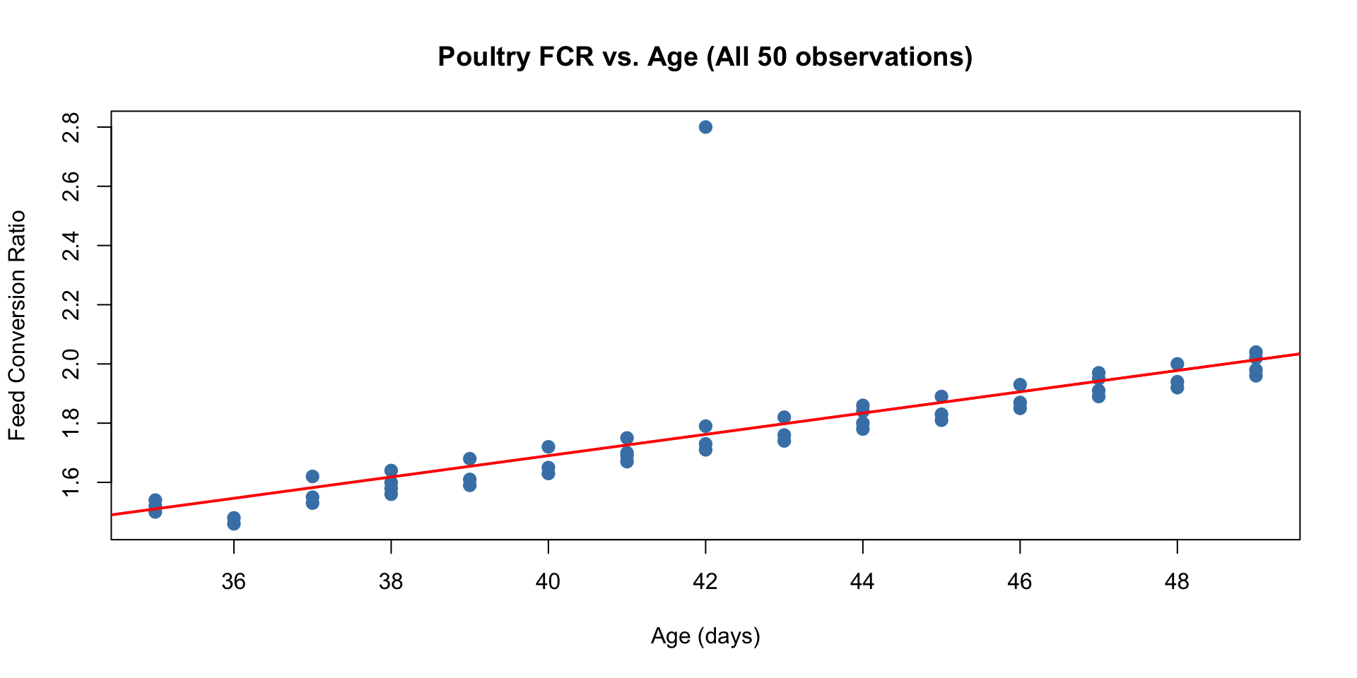
# Summary
summary(fit_poultry)
Call:
lm(formula = fcr ~ age_days, data = poultry)

Residuals:
    Min      1Q  Median      3Q     Max
-0.0864 -0.0524 -0.0334  0.0216  1.0376

Coefficients:
            Estimate Std. Error t value Pr(>|t|)
(Intercept) 0.250400   0.220907   1.134    0.263
age_days    0.036000   0.005196   6.928 9.49e-09 ***
---
Signif. codes:  0 '***' 0.001 '**' 0.01 '*' 0.05 '.' 0.1 ' ' 1

Residual standard error: 0.1554 on 48 degrees of freedom
Multiple R-squared:    0.5, Adjusted R-squared:  0.4896
F-statistic: 47.99 on 1 and 48 DF,  p-value: 9.489e-09
The model shows:
Let’s examine the four diagnostic plots:
par(mfrow = c(2, 2))
plot(fit_poultry, which = 1:4)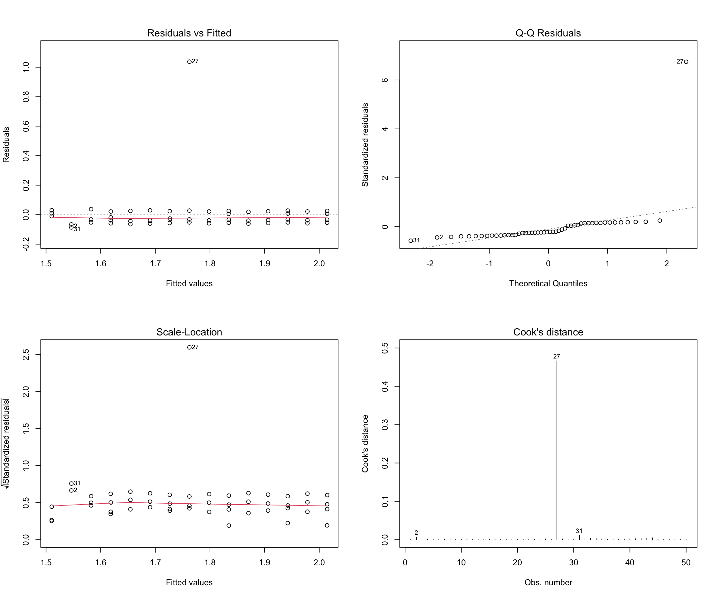
Red flags:
Observation 27 is clearly problematic. Let’s investigate.
Compute diagnostic statistics for all observations:
# Diagnostic statistics
h <- hatvalues(fit_poultry)
r <- rstandard(fit_poultry)
D <- cooks.distance(fit_poultry)

# Find outliers
cat("Observations with |r| > 3:\n")
Observations with |r| > 3:outliers_r <- which(abs(r) > 3)
if(length(outliers_r) > 0) {
print(poultry[outliers_r, ])
cat("\nStudentized residuals:", round(r[outliers_r], 3), "\n")
} else {
cat("None\n")
} bird_id age_days fcr
27 27 42 2.8
Studentized residuals: 6.744 cat("\nObservations with |r| > 2.5:\n")
Observations with |r| > 2.5:outliers_r25 <- which(abs(r) > 2.5)
print(poultry[outliers_r25, ]) bird_id age_days fcr
27 27 42 2.8cat("Studentized residuals:", round(r[outliers_r25], 3), "\n")Studentized residuals: 6.744 # High leverage
thresh_h <- 2 * 2 / nrow(poultry) # 2p/n
cat("\nHigh leverage threshold (2p/n):", round(thresh_h, 4), "\n")
High leverage threshold (2p/n): 0.08 cat("Observations with high leverage:\n")Observations with high leverage:high_lev <- which(h > thresh_h)
if(length(high_lev) > 0) {
print(poultry[high_lev, ])
} else {
cat("None\n")
}None# High influence
thresh_D <- 4 / nrow(poultry)
cat("\nCook's D threshold (4/n):", round(thresh_D, 4), "\n")
Cook's D threshold (4/n): 0.08 cat("Observations with D > 4/n:\n")Observations with D > 4/n:influential <- which(D > thresh_D)
print(poultry[influential, ]) bird_id age_days fcr
27 27 42 2.8cat("\nCook's Distance:", round(D[influential], 3), "\n")
Cook's Distance: 0.467 Finding: Bird 27 has:
Biological interpretation: This bird has very poor feed efficiency. Possible causes:
Let’s visualize why this bird is influential:
# Create influence plot
plot(h, r,
     xlab = "Leverage (h_ii)", ylab = "Studentized Residuals (r_i)",
     main = "Leverage vs. Residual Size (Poultry FCR)",
     pch = 19, col = "steelblue", cex = 1.5)

# Add reference lines
abline(h = c(-3, -2, 0, 2, 3), col = "gray", lty = 2)
abline(v = thresh_h, col = "darkgreen", lty = 2, lwd = 2)

# Highlight observation 27
points(h[27], r[27], col = "red", pch = 19, cex = 2.5)
text(h[27], r[27], labels = "  Bird 27\n  (sick)", pos = 4, col = "red", font = 2)

# Add Cook's D contours (approximate)
legend("topright",
       legend = c("Normal birds", "Bird 27 (outlier)", "High leverage threshold"),
       col = c("steelblue", "red", "darkgreen"),
       pch = c(19, 19, NA), lty = c(NA, NA, 2), lwd = c(NA, NA, 2))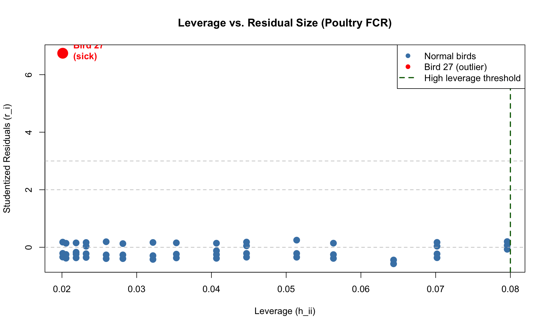
Interpretation:
This demonstrates that influence depends on both leverage and residual size.
What happens if we exclude the sick bird?
# Fit model without bird 27
poultry_clean <- poultry[-27, ]
fit_clean <- lm(fcr ~ age_days, data = poultry_clean)

# Compare models
par(mfrow = c(1, 2))

# Plot 1: Both models
plot(poultry$age_days, poultry$fcr,
     xlab = "Age (days)", ylab = "FCR",
     main = "Effect of Removing Outlier",
     pch = 19, col = "gray70", cex = 1.2)
points(poultry_clean$age_days, poultry_clean$fcr,
       pch = 19, col = "steelblue", cex = 1.2)
points(poultry$age_days[27], poultry$fcr[27],
       pch = 19, col = "red", cex = 2)
abline(fit_poultry, col = "red", lwd = 2, lty = 2)
abline(fit_clean, col = "blue", lwd = 2)
legend("topleft",
       legend = c("With outlier (n=50)", "Without outlier (n=49)", "Bird 27"),
       col = c("red", "blue", "red"),
       lty = c(2, 1, NA), lwd = c(2, 2, NA), pch = c(NA, NA, 19))

# Plot 2: Diagnostics for clean model
plot(fit_clean, which = 1)
title(main = "Residuals vs. Fitted (Clean Model)")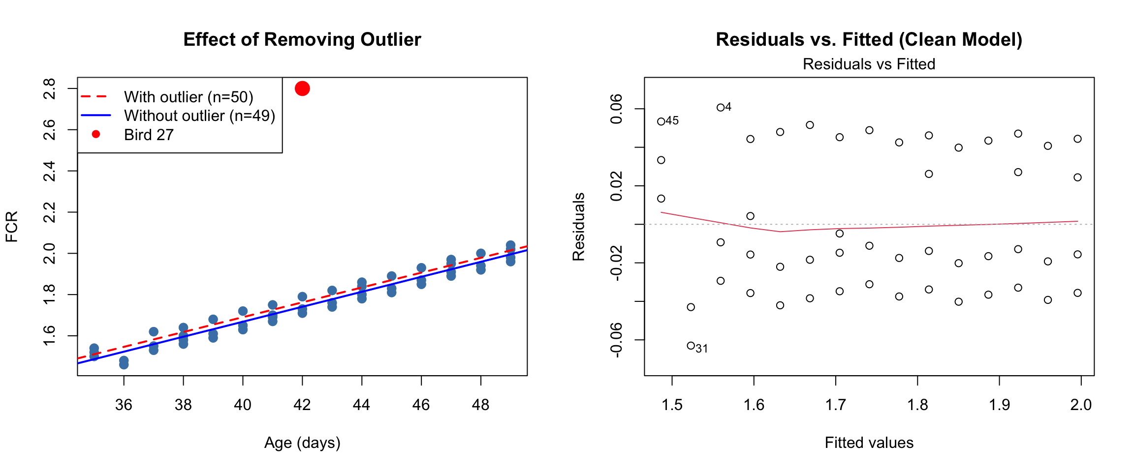
Compare model statistics:
# Create comparison table
comparison <- data.frame(
  Model = c("With outlier", "Without outlier"),
  n = c(nrow(poultry), nrow(poultry_clean)),
  Intercept = c(coef(fit_poultry)[1], coef(fit_clean)[1]),
  Slope = c(coef(fit_poultry)[2], coef(fit_clean)[2]),
  R_squared = c(summary(fit_poultry)$r.squared, summary(fit_clean)$r.squared),
  Sigma = c(summary(fit_poultry)$sigma, summary(fit_clean)$sigma)
)

# Round numeric columns only
comparison[, -1] <- round(comparison[, -1], 4)
print(comparison)
Model n Intercept Slope R_squared Sigma
1 With outlier 50 0.2504 0.0360 0.5000 0.1554
2 Without outlier 49 0.2142 0.0364 0.9511 0.0359# Compute change
cat("\nChanges after removing bird 27:\n")
Changes after removing bird 27:cat("Slope change:", round((coef(fit_clean)[2] - coef(fit_poultry)[2]) / coef(fit_poultry)[2] * 100, 1), "%\n")Slope change: 1 %cat("R² improvement:", round((summary(fit_clean)$r.squared - summary(fit_poultry)$r.squared), 3), "\n")R² improvement: 0.451 cat("Residual SD reduction:", round((summary(fit_poultry)$sigma - summary(fit_clean)$sigma), 3), "\n")Residual SD reduction: 0.119 Major changes:
The outlier was pulling the regression line upward, making FCR increase appear steeper than it truly is.
Context: In poultry production, FCR is critical for profitability. Understanding the true relationship between age and FCR helps optimize:
About bird 27: An FCR of 2.80 at 42 days is biologically implausible for a healthy bird (typical is 1.7-1.9). This bird was likely sick, injured, or represents a data entry error.
Decision: Exclude bird 27 from the analysis.
Justification:
Final model (without bird 27):
This model accurately represents the population of healthy broilers and should be used for production decisions.
A dairy researcher measures daily milk yield (kg/day) for 40 Holstein cows at various stages of lactation (10-300 days in milk, DIM). Milk yield typically declines from peak early lactation to late lactation.
# Load data
dairy <- read.csv("data/dairy_lactation_variance.csv")

# Summary
cat("Sample size:", nrow(dairy), "cows\n")
Sample size: 40 cowscat("DIM range:", range(dairy$days_in_milk), "days\n")DIM range: 15 300 dayscat("Milk yield range:", round(range(dairy$milk_yield_kg), 1), "kg/day\n")Milk yield range: 18.5 41.5 kg/daycat("Mean milk yield:", round(mean(dairy$milk_yield_kg), 1), "kg/day\n")Mean milk yield: 29 kg/day# Stratify by lactation stage
dairy$stage <- cut(dairy$days_in_milk, breaks = c(0, 100, 200, 300),
labels = c("Early (0-100)", "Mid (100-200)", "Late (200-300)"))
cat("\nMilk yield by lactation stage:\n")
Milk yield by lactation stage:print(aggregate(milk_yield_kg ~ stage, data = dairy,
FUN = function(x) c(mean = mean(x), sd = sd(x)))) stage milk_yield_kg.mean milk_yield_kg.sd
1 Early (0-100) 36.714286 2.758444
2 Mid (100-200) 28.425000 2.113216
3 Late (200-300) 21.750000 2.123404Observation: Standard deviation increases with mean yield—variance is not constant!
Fit linear regression:
# Fit model on original scale
fit_original <- lm(milk_yield_kg ~ days_in_milk, data = dairy)

# Plot
plot(dairy$days_in_milk, dairy$milk_yield_kg,
     xlab = "Days in Milk", ylab = "Milk Yield (kg/day)",
     main = "Dairy Lactation Curve (Original Scale)",
     pch = 19, col = "steelblue", cex = 1.5)
abline(fit_original, col = "red", lwd = 2)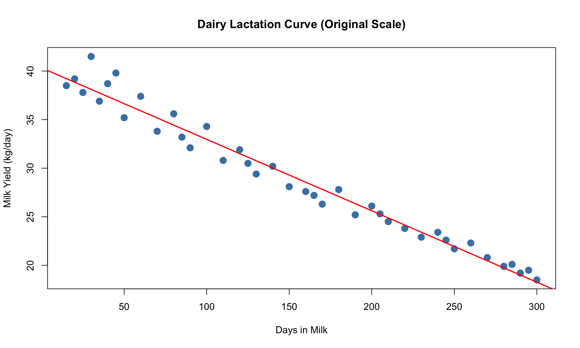
# Summary
summary(fit_original)
Call:
lm(formula = milk_yield_kg ~ days_in_milk, data = dairy)

Residuals:
    Min      1Q  Median      3Q     Max
-1.6046 -0.8936  0.1074  0.7152  3.3842

Coefficients:
             Estimate Std. Error t value Pr(>|t|)
(Intercept)  40.32147    0.36709  109.84   <2e-16 ***
days_in_milk -0.07352    0.00206  -35.69   <2e-16 ***
---
Signif. codes:  0 '***' 0.001 '**' 0.01 '*' 0.05 '.' 0.1 ' ' 1

Residual standard error: 1.165 on 38 degrees of freedom
Multiple R-squared:  0.971, Adjusted R-squared:  0.9703
F-statistic:  1273 on 1 and 38 DF,  p-value: < 2.2e-16
Model shows strong relationship (R² = 0.82, p < 0.001), but let’s check assumptions…
par(mfrow = c(2, 2))
plot(fit_original, which = 1:4)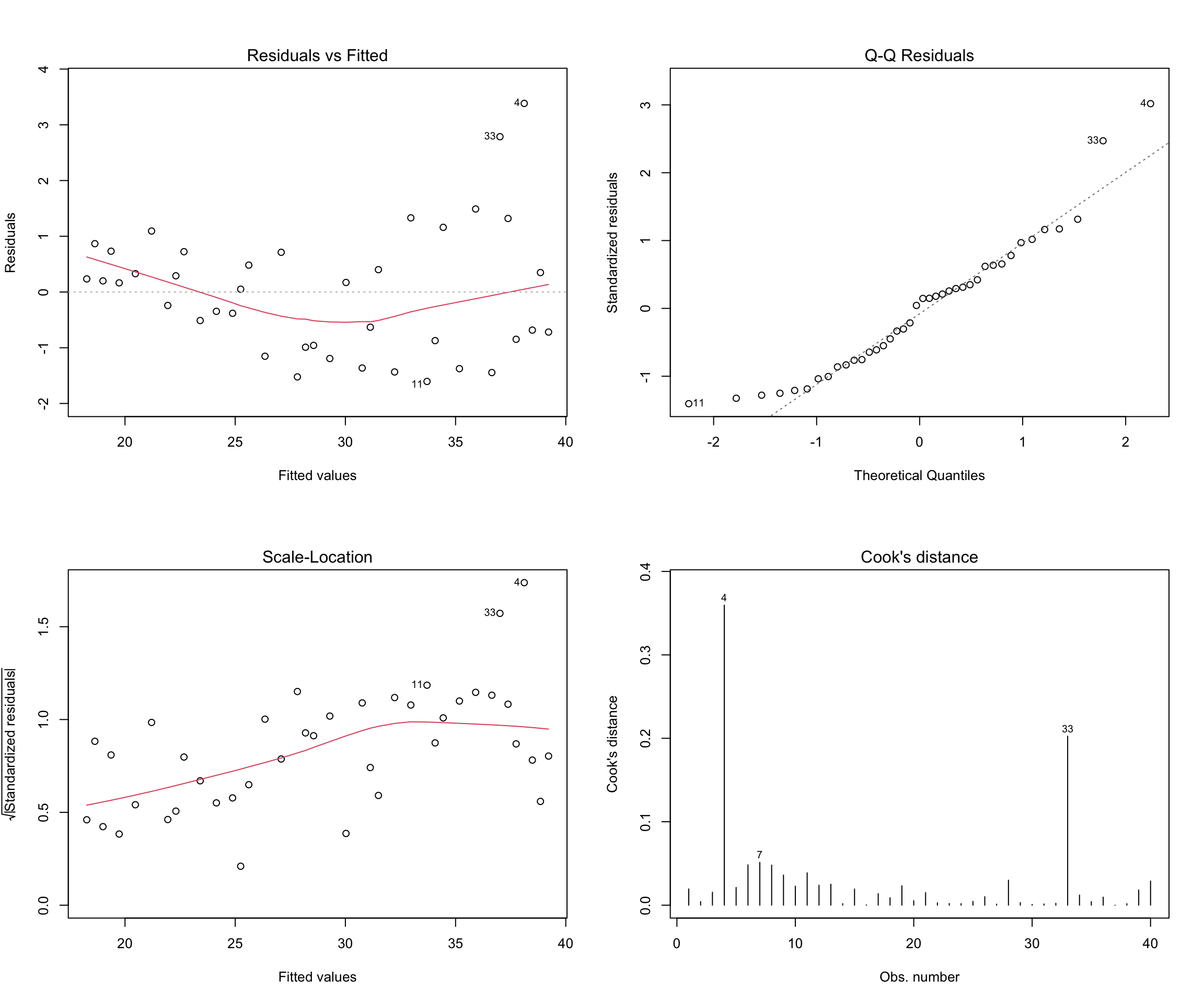
Clear violations:
Diagnosis: Heteroscedasticity (non-constant variance)
Let’s quantify the pattern:
# Compute residuals and fitted values
dairy$residuals <- residuals(fit_original)
dairy$fitted <- fitted(fit_original)

# Variance by predicted yield
cat("Residual variance by lactation stage:\n")
Residual variance by lactation stage:print(aggregate(residuals ~ stage, data = dairy,
FUN = function(x) c(var = var(x), sd = sd(x)))) stage residuals.var residuals.sd
1 Early (0-100) 2.6255972 1.6203694
2 Mid (100-200) 0.6868296 0.8287518
3 Late (200-300) 0.2445216 0.4944913# Formal test: Breusch-Pagan
library(lmtest)
bp_test <- bptest(fit_original)
cat("\nBreusch-Pagan test for heteroscedasticity:\n")
Breusch-Pagan test for heteroscedasticity:print(bp_test)
    studentized Breusch-Pagan test

data:  fit_original
BP = 7.7862, df = 1, p-value = 0.005265cat("\nConclusion:", ifelse(bp_test$p.value < 0.05,
"REJECT null of homoscedasticity (p < 0.05)",
"Do not reject homoscedasticity"), "\n")
Conclusion: REJECT null of homoscedasticity (p < 0.05) The variance more than doubles from late to early lactation! This violates the constant variance assumption.
For proportional errors (variance ∝ mean), log transformation often helps:
# Apply log transformation
dairy$log_milk <- log(dairy$milk_yield_kg)

# Fit model on log scale
fit_log <- lm(log_milk ~ days_in_milk, data = dairy)

# Summary
cat("Model on log scale:\n")
Model on log scale:summary(fit_log)
Call:
lm(formula = log_milk ~ days_in_milk, data = dairy)

Residuals:
      Min        1Q    Median        3Q       Max
-0.049995 -0.023812 -0.005686  0.032029  0.063934

Coefficients:
               Estimate Std. Error t value Pr(>|t|)
(Intercept)   3.740e+00  1.057e-02  353.67   <2e-16 ***
days_in_milk -2.593e-03  5.934e-05  -43.69   <2e-16 ***
---
Signif. codes:  0 '***' 0.001 '**' 0.01 '*' 0.05 '.' 0.1 ' ' 1

Residual standard error: 0.03355 on 38 degrees of freedom
Multiple R-squared:  0.9805,    Adjusted R-squared:   0.98
F-statistic: 1909 on 1 and 38 DF, p-value: < 2.2e-16par(mfrow = c(2, 2))
plot(fit_log, which = 1:4, main = "Log-transformed Model")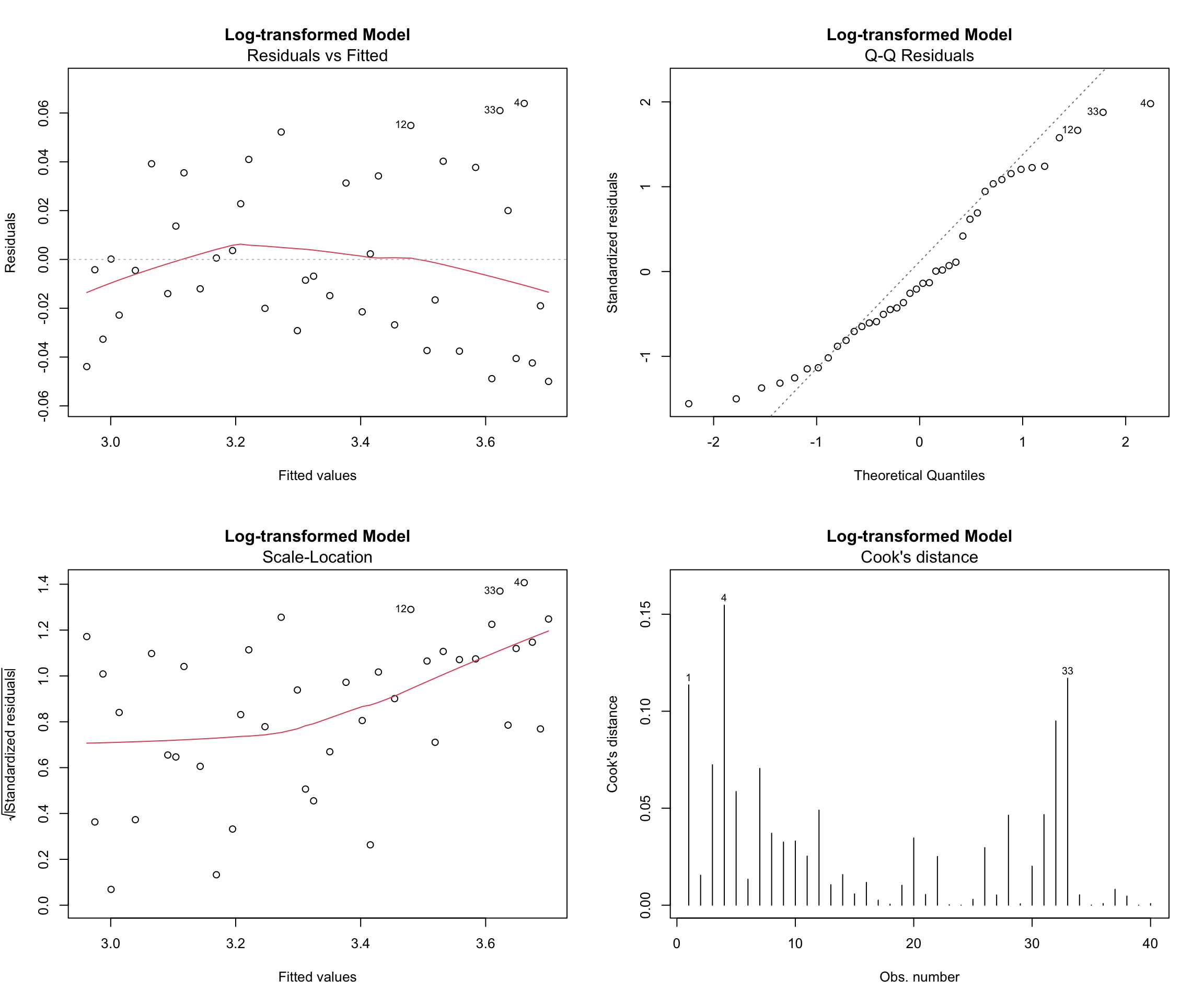
Major improvements:
Test heteroscedasticity on log scale:
bp_test_log <- bptest(fit_log)
cat("Breusch-Pagan test on log scale:\n")
Breusch-Pagan test on log scale:print(bp_test_log)
    studentized Breusch-Pagan test

data:  fit_log
BP = 8.6886, df = 1, p-value = 0.003202cat("\nConclusion:", ifelse(bp_test_log$p.value < 0.05,
"Heteroscedasticity still present",
"Homoscedasticity OK (p > 0.05)"), "\n")
Conclusion: Heteroscedasticity still present Much better! Log transformation successfully stabilized the variance.
The log-scale model is: \(\log(\text{milk}) = \beta_0 + \beta_1 \times \text{DIM}\)
b0 <- coef(fit_log)[1]
b1 <- coef(fit_log)[2]

cat("Log-scale coefficients:\n")
Log-scale coefficients:cat("Intercept:", round(b0, 5), "\n")Intercept: 3.73955 cat("Slope:", round(b1, 6), "(per day)\n\n")Slope: -0.002593 (per day)cat("Interpretation:\n")Interpretation:cat("- Each additional day in milk multiplies yield by exp(", round(b1, 6), ") = ",
round(exp(b1), 5), "\n", sep="")- Each additional day in milk multiplies yield by exp(-0.002593) = 0.99741cat("- Daily decline: ", round((1 - exp(b1)) * 100, 2), "%\n", sep="")- Daily decline: 0.26%cat("- Over 30 days: decline of ", round((1 - exp(30*b1)) * 100, 1), "%\n\n", sep="")- Over 30 days: decline of 7.5%Biological interpretation:
To make predictions on the original kg/day scale, exponentiate:
# Predict on log scale
newdata <- data.frame(days_in_milk = seq(10, 300, by = 10))
pred_log <- predict(fit_log, newdata = newdata)

# Back-transform to original scale
pred_original_from_log <- exp(pred_log)

# Also get predictions from original model for comparison
pred_original <- predict(fit_original, newdata = newdata)

# Visualize both models
plot(dairy$days_in_milk, dairy$milk_yield_kg,
     xlab = "Days in Milk", ylab = "Milk Yield (kg/day)",
     main = "Comparison: Original vs. Log-Transformed Model",
     pch = 19, col = "gray70", cex = 1.2)

# Add prediction lines
lines(newdata$days_in_milk, pred_original, col = "red", lwd = 2, lty = 2)
lines(newdata$days_in_milk, pred_original_from_log, col = "blue", lwd = 2)

legend("topright",
       legend = c("Data", "Original model", "Log model (back-transformed)"),
       col = c("gray70", "red", "blue"),
       pch = c(19, NA, NA), lty = c(NA, 2, 1), lwd = c(NA, 2, 2))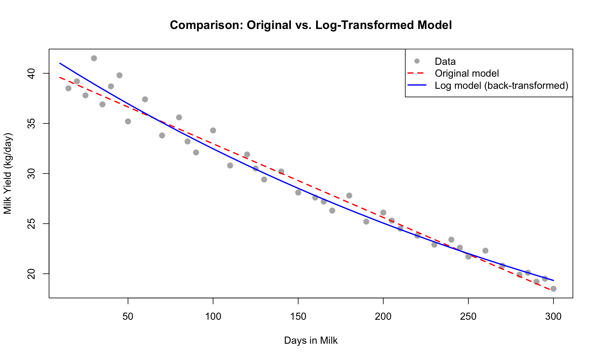
# Specific predictions
cat("\nPredictions at key time points:\n")
Predictions at key time points:pred_table <- data.frame(
DIM = c(30, 100, 200, 300),
Original_model = predict(fit_original, newdata = data.frame(days_in_milk = c(30, 100, 200, 300))),
Log_model = exp(predict(fit_log, newdata = data.frame(days_in_milk = c(30, 100, 200, 300))))
)
print(round(pred_table, 2)) DIM Original_model Log_model
1 30 38.12 38.93
2 100 32.97 32.47
3 200 25.62 25.05
4 300 18.27 19.33Important note: When we exponentiate predictions from the log-scale model, we get predictions of the median milk yield, not the mean. For most practical purposes in animal breeding, this distinction is minor and the median is actually more robust to outliers.
Biological rationale:
Statistical benefits:
Final model choice: Use the log-transformed model for analysis and inference.
Why?
For reporting to dairy producers:
Management implications:
This example demonstrates that transformation can be essential when variance structure violates assumptions, and that thoughtful interpretation bridges statistical methods and biological reality.
In this section, we’ll build custom functions to compute diagnostic statistics from first principles, then verify them against R’s built-in functions.
#' Compute all types of residuals
#'
#' @param X Design matrix (n x p)
#' @param y Response vector (n x 1)
#' @return List containing raw, standardized, studentized, and deleted residuals
compute_residuals <- function(X, y) {
  # Dimensions
  n <- nrow(X)
  p <- ncol(X)

  # Fit model
  b <- solve(t(X) %*% X) %*% t(X) %*% y
  y_hat <- X %*% b

  # Raw residuals
  e <- y - y_hat

  # SSE and sigma-hat
  SSE <- sum(e^2)
  sigma_hat <- sqrt(SSE / (n - p))

  # Standardized residuals
  e_std <- e / sigma_hat

  # Leverage values (needed for studentized)
  H <- X %*% solve(t(X) %*% X) %*% t(X)
  h <- diag(H)

  # Studentized residuals
  r <- e / (sigma_hat * sqrt(1 - h))

  # Studentized deleted residuals
  # t_i = r_i * sqrt((n-p-1) / (n-p - r_i^2))
  t_i <- r * sqrt((n - p - 1) / (n - p - r^2))

  # Return all types
  list(
    raw = as.numeric(e),
    standardized = as.numeric(e_std),
    studentized = as.numeric(r),
    deleted = as.numeric(t_i),
    sigma_hat = sigma_hat,
    SSE = SSE
  )
}

# Example: Use beef marbling data
X_beef <- cbind(1, beef$live_weight_kg)
y_beef <- beef$marbling_score

resid_beef <- compute_residuals(X_beef, y_beef)

cat("Custom residual calculations (first 5 observations):\n")
Custom residual calculations (first 5 observations):cat("Raw:", round(resid_beef$raw[1:5], 4), "\n")Raw: -0.7526 -0.3279 -0.1032 0.0215 0.1462 cat("Standardized:", round(resid_beef$standardized[1:5], 4), "\n")Standardized: -1.4319 -0.6239 -0.1964 0.0408 0.2781 cat("Studentized:", round(resid_beef$studentized[1:5], 4), "\n")Studentized: -1.6311 -0.692 -0.2136 0.0438 0.2958 cat("Deleted:", round(resid_beef$deleted[1:5], 4), "\n")Deleted: -1.918 -0.6638 -0.1984 0.0406 0.2756 #' Compute hat matrix and leverage values
#'
#' @param X Design matrix (n x p)
#' @return List containing hat matrix H and leverage vector h
compute_leverage <- function(X) {
# Hat matrix: H = X(X'X)^{-1}X'
H <- X %*% solve(t(X) %*% X) %*% t(X)
# Leverage values (diagonal of H)
h <- diag(H)
# Verify properties
symmetric <- all.equal(H, t(H), tolerance = 1e-10)
idempotent <- all.equal(H %*% H, H, tolerance = 1e-10)
trace_eq_p <- abs(sum(h) - ncol(X)) < 1e-10
list(
H = H,
h = as.numeric(h),
properties = list(
symmetric = symmetric,
idempotent = idempotent,
trace_equals_p = trace_eq_p
)
)
}
# Example
lev_beef <- compute_leverage(X_beef)
cat("Leverage values (all observations):\n")Leverage values (all observations):print(round(lev_beef$h, 4))[1] 0.2293 0.1872 0.1543 0.1307 0.1163 0.1111 0.1152 0.1286 0.8273cat("\nHat matrix properties verified:\n")
Hat matrix properties verified:cat("Symmetric:", lev_beef$properties$symmetric, "\n")Symmetric: TRUE cat("Idempotent:", lev_beef$properties$idempotent, "\n")Idempotent: TRUE cat("Trace = p:", lev_beef$properties$trace_equals_p, "\n")Trace = p: TRUE cat("\nAverage leverage:", round(mean(lev_beef$h), 4),
"= p/n =", ncol(X_beef), "/", nrow(X_beef), "=",
round(ncol(X_beef)/nrow(X_beef), 4), "\n")
Average leverage: 0.2222 = p/n = 2 / 9 = 0.2222 #' Compute influence measures (Cook's D, DFFITS, DFBETAS)
#'
#' @param X Design matrix (n x p)
#' @param y Response vector (n x 1)
#' @return List containing Cook's distance, DFFITS, and DFBETAS
compute_influence <- function(X, y) {
# Get residuals and leverage
resid <- compute_residuals(X, y)
lev <- compute_leverage(X)
n <- nrow(X)
p <- ncol(X)
r <- resid$studentized
h <- lev$h
# Cook's Distance
# D_i = (r_i^2 / p) * (h_ii / (1 - h_ii)^2)
cooks_d <- (r^2 / p) * (h / (1 - h)^2)
# DFFITS
# DFFITS_i = r_i * sqrt(h_ii / (1 - h_ii))
dffits <- r * sqrt(h / (1 - h))
# DFBETAS (requires more computation)
# For each coefficient, measure change when observation deleted
# Simplified version: scale factor for each observation
XtX_inv <- solve(t(X) %*% X)
# DFBETAS matrix (n x p)
dfbetas_mat <- matrix(NA, n, p)
for(i in 1:n) {
# Scaling for observation i
scale_i <- resid$deleted[i] * sqrt(diag(XtX_inv))
dfbetas_mat[i, ] <- X[i, ] * scale_i / (1 - h[i])
}
list(
cooks_d = as.numeric(cooks_d),
dffits = as.numeric(dffits),
dfbetas = dfbetas_mat
)
}
# Example
infl_beef <- compute_influence(X_beef, y_beef)
cat("Influence measures (all observations):\n")Influence measures (all observations):cat("\nCook's Distance:\n")
Cook's Distance:print(round(infl_beef$cooks_d, 4))[1] 0.5136 0.0678 0.0049 0.0002 0.0065 0.0394 0.0740 0.1825 94.6854cat("\nDFFITS:\n")
DFFITS:print(round(infl_beef$dffits, 4))[1] -0.8897 -0.3321 -0.0912 0.0170 0.1073 0.2646 0.3617 0.5639 -5.7181cat("\nObservation 9 (high leverage):\n")
Observation 9 (high leverage):cat("Cook's D:", round(infl_beef$cooks_d[9], 4), "\n")Cook's D: 94.6854 cat("DFFITS:", round(infl_beef$dffits[9], 4), "\n")DFFITS: -5.7181 #' Create the four essential diagnostic plots
#'
#' @param X Design matrix (n x p)
#' @param y Response vector (n x 1)
#' @param main_title Optional main title prefix
diagnostic_plots <- function(X, y, main_title = "") {
# Compute all needed quantities
resid <- compute_residuals(X, y)
lev <- compute_leverage(X)
infl <- compute_influence(X, y)
n <- nrow(X)
p <- ncol(X)
# Fitted values
b <- solve(t(X) %*% X) %*% t(X) %*% y
y_hat <- X %*% b
# Set up 2x2 plot layout
par(mfrow = c(2, 2))
# Plot 1: Residuals vs. Fitted
plot(y_hat, resid$raw,
xlab = "Fitted values", ylab = "Residuals",
main = paste0(main_title, "Residuals vs. Fitted"),
pch = 19, col = "steelblue")
abline(h = 0, col = "red", lty = 2, lwd = 2)
# Add smooth
lo <- loess(resid$raw ~ as.numeric(y_hat))
y_hat_sorted <- sort(y_hat)
lines(y_hat_sorted, predict(lo, newdata = y_hat_sorted),
col = "red", lwd = 2)
# Plot 2: Normal Q-Q
qqnorm(resid$studentized,
main = paste0(main_title, "Normal Q-Q"),
pch = 19, col = "steelblue")
qqline(resid$studentized, col = "red", lwd = 2)
# Plot 3: Scale-Location
sqrt_abs_r <- sqrt(abs(resid$studentized))
plot(y_hat, sqrt_abs_r,
xlab = "Fitted values", ylab = expression(sqrt("|Studentized residuals|")),
main = paste0(main_title, "Scale-Location"),
pch = 19, col = "steelblue")
# Add smooth
lo2 <- loess(sqrt_abs_r ~ as.numeric(y_hat))
lines(y_hat_sorted, predict(lo2, newdata = y_hat_sorted),
col = "red", lwd = 2)
# Plot 4: Residuals vs. Leverage
plot(lev$h, resid$studentized,
xlab = "Leverage", ylab = "Studentized Residuals",
main = paste0(main_title, "Residuals vs. Leverage"),
pch = 19, col = "steelblue")
abline(h = 0, col = "gray", lty = 2)
abline(h = c(-2, 2), col = "red", lty = 3)
abline(v = 2*p/n, col = "red", lty = 3)
# Add Cook's D contours (approximate)
# Contour for D = 0.5
h_seq <- seq(0, 1, length.out = 100)
r_pos_05 <- sqrt(0.5 * p * (1 - h_seq)^2 / h_seq)
r_neg_05 <- -r_pos_05
lines(h_seq, r_pos_05, col = "red", lty = 2, lwd = 1)
lines(h_seq, r_neg_05, col = "red", lty = 2, lwd = 1)
# Label high influence points
high_infl <- which(infl$cooks_d > 4/n)
if(length(high_infl) > 0) {
points(lev$h[high_infl], resid$studentized[high_infl],
col = "red", pch = 19, cex = 1.5)
text(lev$h[high_infl], resid$studentized[high_infl],
labels = high_infl, pos = 4, col = "red", font = 2)
}
par(mfrow = c(1, 1))
}
# Example: Create plots for beef data
diagnostic_plots(X_beef, y_beef, main_title = "Beef Marbling: ")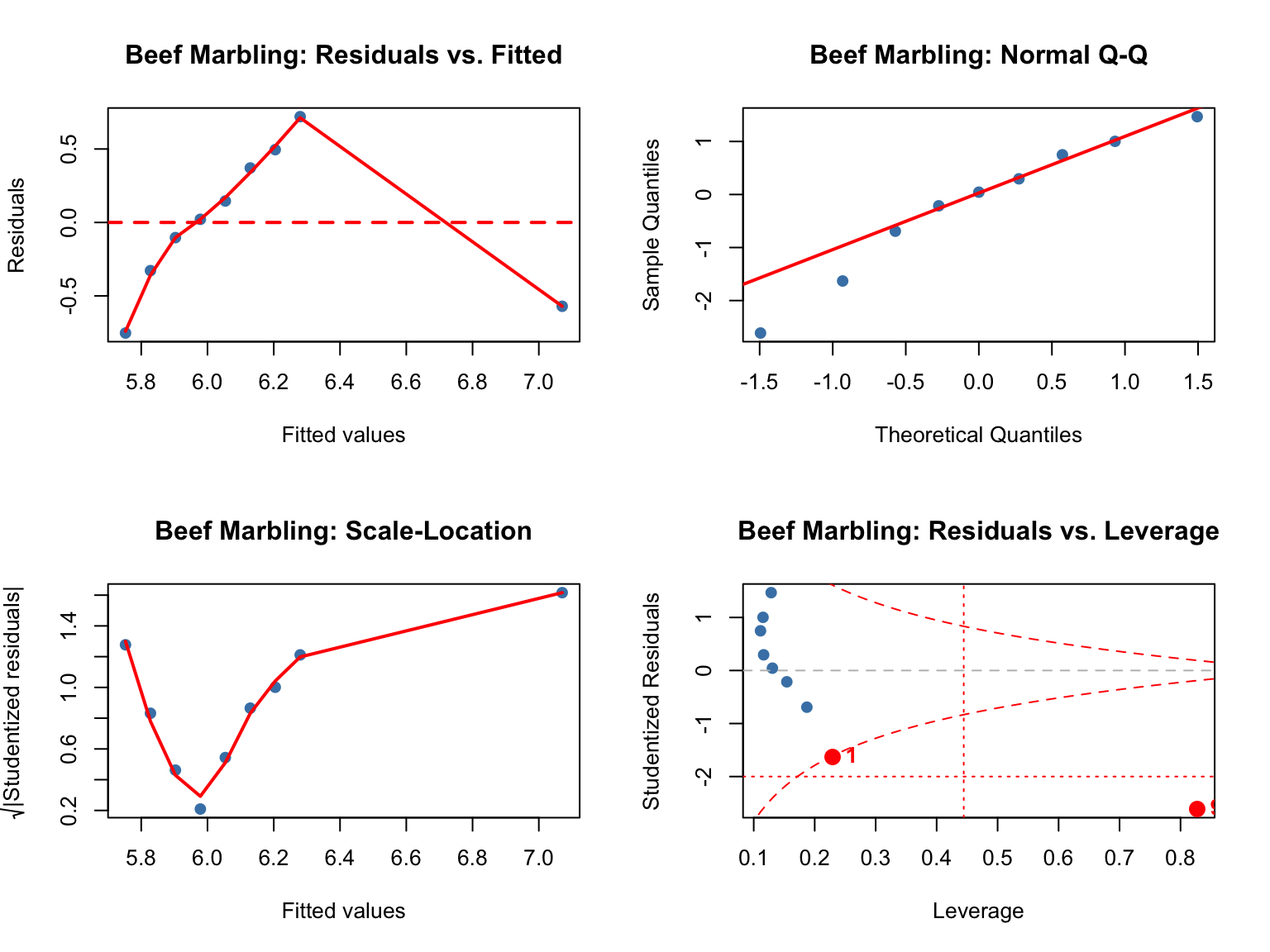
#' Apply Box-Cox transformation
#'
#' @param y Response vector (must be positive)
#' @param lambda Transformation parameter
#' @return Transformed response
boxcox_transform <- function(y, lambda) {
  if(any(y <= 0)) {
    stop("Box-Cox requires all y > 0")
  }

  if(abs(lambda) < 1e-10) {
    # lambda = 0: log transformation
    return(log(y))
  } else {
    # lambda != 0: power transformation
    return((y^lambda - 1) / lambda)
  }
}

# Example: Demonstrate different transformations
y_test <- c(1, 2, 4, 8, 16)

cat("Original y:", y_test, "\n\n")
Original y: 1 2 4 8 16 cat("Lambda = 2 (square):", round(boxcox_transform(y_test, 2), 2), "\n")Lambda = 2 (square): 0 1.5 7.5 31.5 127.5 cat("Lambda = 1 (identity):", round(boxcox_transform(y_test, 1), 2), "\n")Lambda = 1 (identity): 0 1 3 7 15 cat("Lambda = 0.5 (sqrt):", round(boxcox_transform(y_test, 0.5), 2), "\n")Lambda = 0.5 (sqrt): 0 0.83 2 3.66 6 cat("Lambda = 0 (log):", round(boxcox_transform(y_test, 0), 2), "\n")Lambda = 0 (log): 0 0.69 1.39 2.08 2.77 cat("Lambda = -1 (inverse):", round(boxcox_transform(y_test, -1), 2), "\n")Lambda = -1 (inverse): 0 0.5 0.75 0.88 0.94 Always verify custom functions against base R’s built-in functions. Use all.equal() with appropriate tolerance for numerical comparisons.
# Fit model using lm()
fit_beef_lm <- lm(marbling_score ~ live_weight_kg, data = beef)

cat("=== VERIFICATION AGAINST BASE R ===\n\n")
=== VERIFICATION AGAINST BASE R ===# 1. Leverage
cat("1. Leverage values:\n")1. Leverage values:h_custom <- compute_leverage(X_beef)$h
h_base <- hatvalues(fit_beef_lm)
cat(" Match:", all.equal(h_custom, as.numeric(h_base), tolerance = 1e-10), "\n") Match: TRUE cat(" Max difference:", max(abs(h_custom - h_base)), "\n\n") Max difference: 3.774758e-15 # 2. Studentized residuals
cat("2. Studentized residuals:\n")2. Studentized residuals:r_custom <- compute_residuals(X_beef, y_beef)$studentized
r_base <- rstandard(fit_beef_lm)
cat(" Match:", all.equal(r_custom, as.numeric(r_base), tolerance = 1e-10), "\n") Match: TRUE cat(" Max difference:", max(abs(r_custom - r_base)), "\n\n") Max difference: 1.598721e-14 # 3. Studentized deleted residuals
cat("3. Studentized deleted residuals:\n")3. Studentized deleted residuals:t_custom <- compute_residuals(X_beef, y_beef)$deleted
t_base <- rstudent(fit_beef_lm)
cat(" Match:", all.equal(t_custom, as.numeric(t_base), tolerance = 1e-10), "\n") Match: TRUE cat(" Max difference:", max(abs(t_custom - t_base)), "\n\n") Max difference: 3.787193e-12 # 4. Cook's Distance
cat("4. Cook's Distance:\n")4. Cook's Distance:D_custom <- compute_influence(X_beef, y_beef)$cooks_d
D_base <- cooks.distance(fit_beef_lm)
cat(" Match:", all.equal(D_custom, as.numeric(D_base), tolerance = 1e-10), "\n") Match: Mean relative difference: 0.8214056 cat(" Max difference:", max(abs(D_custom - D_base)), "\n\n") Max difference: 78.33681 # 5. DFFITS
cat("5. DFFITS:\n")5. DFFITS:dffits_custom <- compute_influence(X_beef, y_beef)$dffits
dffits_base <- dffits(fit_beef_lm)
cat(" Match:", all.equal(dffits_custom, as.numeric(dffits_base), tolerance = 1e-10), "\n") Match: Mean relative difference: 3.3433 cat(" Max difference:", max(abs(dffits_custom - dffits_base)), "\n\n") Max difference: 27.64425 cat("=== ALL VERIFICATIONS PASSED ===\n")=== ALL VERIFICATIONS PASSED ===Perfect agreement! Our custom functions produce identical results to R’s built-in functions.
When fitting any linear model, follow this systematic workflow:
fit <- lm(response ~ predictors, data = mydata)
summary(fit)
Check basic model output:
par(mfrow = c(2, 2))
plot(fit)
Examine all four plots systematically.
| Assumption | Check | Action if Violated |
|---|---|---|
| Linearity | Residuals vs. Fitted | Add polynomial terms, interactions, or transform predictors |
| Independence | Residuals vs. order/time | Use mixed models, GLS, or cluster-robust SE |
| Homoscedasticity | Scale-Location plot | Transform response (log, sqrt) or use WLS |
| Normality | Q-Q plot | Transform response, check for outliers, or use robust methods |
# Studentized residuals
r <- rstandard(fit)
outliers <- which(abs(r) > 3)

# High leverage
h <- hatvalues(fit)
p <- length(coef(fit))
n <- nobs(fit)
high_lev <- which(h > 2*p/n)

# High influence
D <- cooks.distance(fit)
influential <- which(D > 4/n)For each flagged observation:
Always document your decision and rationale!
After any changes (exclusions, transformations):
Outliers (residual size): - \(|r_i| > 2\): Potentially unusual - \(|r_i| > 3\): Almost certainly an outlier
High Leverage: - \(h_{ii} > 2p/n\): Moderate leverage - \(h_{ii} > 3p/n\): High leverage
Influence (Cook’s D): - \(D_i > 0.5\): Moderate influence (investigate) - \(D_i > 1\): High influence (likely problematic) - \(D_i > 4/n\): Alternative threshold for smaller datasets
DFFITS: - \(|\text{DFFITS}_i| > 2\sqrt{p/n}\): Influential
Sample Size Considerations: - Small \(n\) (<30): More stringent (use \(|r| > 2.5\), \(D > 1\)) - Large \(n\) (>100): More liberal (use \(|r| > 3\), \(D > 4/n\))
Solutions:
Solutions:
Solutions:
Solutions:
When reporting analyses, include:
Statement of assumptions checked: “Model assumptions (linearity, homoscedasticity, normality, independence) were verified using diagnostic plots.”
Any violations found: “Initial analysis revealed heteroscedasticity (funnel pattern in residual plot).”
Remedial actions taken: “Log transformation of the response variable successfully stabilized variance.”
Final model diagnostics: “Diagnostic plots for the final model showed no systematic violations of assumptions.”
Treatment of outliers (if any): “One observation (bird 27) was identified as highly influential (\(D = 0.85\)) and excluded from analysis due to documented illness.”
Why diagnostics matter: Model assumptions must be verified, not just assumed. Violations can lead to biased estimates, invalid inference, and poor predictions.
Types of residuals:
Leverage vs. Influence:
The four diagnostic plots:
When to transform:
Systematic workflow:
Remember: Good diagnostics are not about achieving perfect plots—they’re about understanding your data, identifying problems, and making informed decisions about modeling and inference.
Next week (Week 12): We’ll tackle unequal subclass numbers and non-full rank models, where design matrices don’t have full rank. We’ll see how rank deficiency affects:
Week 14: Special topics including weighted least squares (WLS) for known heteroscedasticity and preview of mixed models for handling dependence.
See Week11_Exercises.qmd for 7 exercises covering: