---
title: "Week 9: Two-Way ANOVA and Factorial Models"
format:
html:
toc: true
toc-depth: 3
number-sections: true
code-fold: false
code-tools: true
bibliography: ../references.bib
---
::: {.callout-note icon=false}
## Learning Objectives
By the end of this week, you will be able to:
1. **Build** and **interpret** **two-way ANOVA models** with **interaction effects** in the context of animal breeding and genetics
2. **Construct** **design matrices** for **factorial designs** (both balanced and unbalanced) and understand their **rank properties**
3. **Compute** and **interpret** **Type I**, **Type II**, and **Type III sums of squares**, and understand when each is appropriate
4. **Test** hypotheses about **main effects** and **interactions** using **F-tests** and interpret results biologically
5. **Conduct** **simple effects analysis** when interactions are significant to understand effect patterns
:::
---
# Introduction
## Why Learn Two-Way ANOVA?
In Week 7, we learned how to compare groups using one-way ANOVA—testing whether a single factor (like breed or diet) affects an outcome. But in animal breeding and production, we often need to study **two or more factors simultaneously**. More importantly, we need to understand whether factors **interact** with each other.
**Real-world examples from animal agriculture:**
1. **Genotype × Environment Interactions**: A beef breed that performs exceptionally well in one production system (e.g., feedlot) may not excel in another (e.g., grass-fed). Selection programs must account for these interactions.
2. **Breed × Sex Effects**: Male and female animals within the same breed may respond differently to genetic selection or management practices. Growth rates, carcass composition, and reproductive traits often show sex-specific patterns.
3. **Diet × Genetic Line Interactions**: Some pig genetic lines respond dramatically to improved nutrition (high lean growth potential), while others show more modest responses. Matching genetics to feeding strategy is economically critical.
4. **Treatment × Time Interactions**: The effectiveness of a health intervention may vary across different stages of production or ages of animals.
::: {.callout-important}
## Interactions Change Everything
An **interaction** occurs when the effect of one factor depends on the level of another factor. When an interaction is present, we cannot simply interpret main effects in isolation—the story is more complex and usually more interesting biologically.
**Example**: If Duroc pigs gain 0.10 kg/day more than Yorkshire on Diet 1, but 0.25 kg/day more on Diet 2, there's a breed × diet interaction. The breed difference isn't constant across diets.
:::
## Connection to Week 7
Week 7 introduced one-way ANOVA with a single factor. This week, we **extend** that framework to two factors:
| Aspect | One-Way ANOVA (Week 7) | Two-Way ANOVA (Week 9) |
|--------|------------------------|------------------------|
| Number of factors | 1 | 2 |
| Model | $y_{ij} = \mu + \alpha_i + e_{ij}$ | $y_{ijk} = \mu + \alpha_i + \beta_j + (\alpha\beta)_{ij} + e_{ijk}$ |
| Effects tested | One main effect | Two main effects + interaction |
| Design matrix | Indicators for one factor | Indicators for two factors + products |
| Interpretation | Group differences | Main effects + interactions |
The mathematical principles remain the same (least squares, normal equations, F-tests), but the model becomes richer and more realistic.
## Preview: What We'll Cover
1. **Mathematical Foundation**: The two-way ANOVA model, both effects and cell means parameterizations
2. **Sum of Squares Decomposition**: Partitioning variation among main effects, interaction, and error
3. **Type I, II, and III SS**: Why different approaches exist and when each matters (critical for unbalanced data!)
4. **Interaction Interpretation**: How to visualize and understand when effects depend on other factors
5. **Simple Effects Analysis**: Decomposing significant interactions to understand patterns
6. **Effect Sizes**: Quantifying practical significance beyond p-values
7. **R Implementation**: Building a complete two-way ANOVA solver from scratch
::: {.callout-note}
## The Two-Way ANOVA Table Structure
We'll partition total variation into **four components** instead of two:
- **SS(Factor A)**: Variation explained by first factor (e.g., breed)
- **SS(Factor B)**: Variation explained by second factor (e.g., diet)
- **SS(A×B)**: Variation explained by interaction between factors
- **SSE**: Residual variation within cells
Total: $SST = SS(A) + SS(B) + SS(AB) + SSE$ (for balanced designs)
:::
---
# Mathematical Theory
## The Two-Way ANOVA Model
### Effects Model (Overparameterized)
The **effects model** for two-way ANOVA with interaction is:
$$
y_{ijk} = \mu + \alpha_i + \beta_j + (\alpha\beta)_{ij} + e_{ijk}
$$ {#eq-twoway-effects}
where:
- $y_{ijk}$ is the $k$-th observation in cell $(i,j)$ (scalar)
- $\mu$ is the overall mean (scalar)
- $\alpha_i$ is the effect of level $i$ of Factor A (scalar), $i = 1, \ldots, a$
- $\beta_j$ is the effect of level $j$ of Factor B (scalar), $j = 1, \ldots, b$
- $(\alpha\beta)_{ij}$ is the interaction effect for cell $(i,j)$ (scalar)
- $e_{ijk}$ is the random error (scalar), $k = 1, \ldots, n_{ij}$
- $n_{ij}$ is the number of observations in cell $(i,j)$
- $N = \sum_{i=1}^{a} \sum_{j=1}^{b} n_{ij}$ is the total sample size
::: {.callout-note}
## Notation and Dimensions
**Scalar quantities**:
- $a$: number of levels of Factor A
- $b$: number of levels of Factor B
- $n_{ij}$: replicates in cell $(i,j)$
- $N$: total observations
**Response vector**:
- **y**: $N \times 1$ vector of all observations
**Parameter vector** (effects model):
- **β**: $(1 + a + b + ab) \times 1$ vector: $[\mu, \alpha_1, \ldots, \alpha_a, \beta_1, \ldots, \beta_b, (\alpha\beta)_{11}, \ldots, (\alpha\beta)_{ab}]'$
**Design matrix** (effects model):
- **X**: $N \times (1 + a + b + ab)$ matrix (usually not full rank)
:::
### Constraints for Identifiability
The effects model in @eq-twoway-effects is **overparameterized**—there are more parameters than we can uniquely estimate. We need constraints to achieve a unique solution.
**Standard sum-to-zero constraints**:
$$
\sum_{i=1}^{a} \alpha_i = 0, \quad \sum_{j=1}^{b} \beta_j = 0
$$ {#eq-main-constraints}
$$
\sum_{i=1}^{a} (\alpha\beta)_{ij} = 0 \text{ for all } j, \quad \sum_{j=1}^{b} (\alpha\beta)_{ij} = 0 \text{ for all } i
$$ {#eq-interaction-constraints}
These constraints ensure:
- Main effects represent deviations from the overall mean
- Interaction effects sum to zero across each factor
- Parameters are uniquely estimable under these restrictions
**Alternative: Reference cell parameterization** (R default with `lm()`):
- Set $\alpha_1 = 0$ and $\beta_1 = 0$ (first level is reference)
- Interpret other $\alpha_i$ and $\beta_j$ as deviations from reference
- Set $(\alpha\beta)_{1j} = 0$ and $(\alpha\beta)_{i1} = 0$
Both approaches lead to the same fitted values and hypothesis tests for **estimable functions**.
### Cell Means Model (Always Full Rank)
An alternative parameterization that avoids overparameterization is the **cell means model**:
$$
y_{ijk} = \mu_{ij} + e_{ijk}
$$ {#eq-cell-means}
where:
- $\mu_{ij}$ is the mean for cell $(i,j)$ (scalar)
- $i = 1, \ldots, a$; $j = 1, \ldots, b$; $k = 1, \ldots, n_{ij}$
**Advantages of cell means model**:
- Design matrix **X** is always full rank: $N \times ab$
- All cell means $\mu_{ij}$ are directly estimable
- No constraints needed
- Easier to work with for unbalanced designs
**Relationship to effects model**:
$$
\mu_{ij} = \mu + \alpha_i + \beta_j + (\alpha\beta)_{ij}
$$ {#eq-cell-means-relationship}
The cell means model is often easier for computation, while the effects model is more interpretable for hypothesis testing about main effects and interactions.
## Matrix Representation
### Effects Model Design Matrix
For a 2×2 factorial (Factor A with 2 levels, Factor B with 2 levels, $n$ observations per cell), using **sum-to-zero constraints**, a typical row of **X** for observation in cell $(i,j)$ looks like:
$$
\mathbf{X} = \begin{bmatrix}
1 & x_{A1} & x_{B1} & x_{AB11} \\
1 & x_{A1} & x_{B2} & x_{AB12} \\
\vdots & \vdots & \vdots & \vdots
\end{bmatrix}
$$
where the coding depends on the chosen constraints. With sum-to-zero constraints:
- Intercept column: all 1's
- Factor A columns: effects coding ($-1, 1$ for 2 levels)
- Factor B columns: effects coding ($-1, 1$ for 2 levels)
- Interaction columns: products of A and B codings
**For reference cell coding** (R default):
- Level 1 of each factor is omitted (implicit reference)
- Other levels coded as 0/1 indicators
- Interactions are products of these indicators
::: {.callout-warning}
## Rank Deficiency Alert
With effects parameterization and no constraints, **X'X** is **singular** (not full rank). The normal equations $\mathbf{X'Xb} = \mathbf{X'y}$ have infinitely many solutions.
To obtain a unique solution, we either:
1. Impose constraints (sum-to-zero or set-to-zero)
2. Use a generalized inverse
3. Switch to cell means parameterization
:::
### Cell Means Design Matrix
For the same 2×2 factorial with cell means model, **X** is simpler:
$$
\mathbf{X} = \begin{bmatrix}
1 & 0 & 0 & 0 \\
1 & 0 & 0 & 0 \\
0 & 1 & 0 & 0 \\
0 & 1 & 0 & 0 \\
0 & 0 & 1 & 0 \\
0 & 0 & 1 & 0 \\
0 & 0 & 0 & 1 \\
0 & 0 & 0 & 1
\end{bmatrix}_{8 \times 4}
$$
Each column is an indicator for one of the $ab = 4$ cells. This matrix is **full rank** ($r(\mathbf{X}) = 4$).
### Normal Equations
For both parameterizations, we minimize the sum of squared errors:
$$
SSE = (\mathbf{y} - \mathbf{Xβ})'(\mathbf{y} - \mathbf{Xβ})
$$
Taking derivatives and setting to zero yields the **normal equations**:
$$
\mathbf{X'Xb} = \mathbf{X'y}
$$ {#eq-normal-equations}
- **Cell means model**: $\mathbf{X'X}$ is full rank → unique solution $\mathbf{b} = (\mathbf{X'X})^{-1}\mathbf{X'y}$
- **Effects model**: $\mathbf{X'X}$ is singular → use generalized inverse $\mathbf{b} = (\mathbf{X'X})^{-}\mathbf{X'y}$ (not unique) or impose constraints
## Sum of Squares Decomposition (Balanced Design)
For a **balanced design** where $n_{ij} = n$ for all cells (equal replication):
### Notation for Means
Let:
- $\bar{y}_{ij.} = \frac{1}{n}\sum_{k=1}^{n} y_{ijk}$ = mean of cell $(i,j)$
- $\bar{y}_{i..} = \frac{1}{bn}\sum_{j=1}^{b}\sum_{k=1}^{n} y_{ijk}$ = marginal mean for level $i$ of Factor A
- $\bar{y}_{.j.} = \frac{1}{an}\sum_{i=1}^{a}\sum_{k=1}^{n} y_{ijk}$ = marginal mean for level $j$ of Factor B
- $\bar{y}_{...} = \frac{1}{abn}\sum_{i=1}^{a}\sum_{j=1}^{b}\sum_{k=1}^{n} y_{ijk}$ = grand mean
### Sum of Squares Formulas
The total sum of squares is:
$$
SST = \sum_{i=1}^{a}\sum_{j=1}^{b}\sum_{k=1}^{n} (y_{ijk} - \bar{y}_{...})^2
$$ {#eq-sst}
which can be partitioned into four components:
**Sum of squares for Factor A (Main Effect)**:
$$
SS(A) = bn \sum_{i=1}^{a} (\bar{y}_{i..} - \bar{y}_{...})^2
$$ {#eq-ssa}
This measures variation in marginal means for Factor A.
**Sum of squares for Factor B (Main Effect)**:
$$
SS(B) = an \sum_{j=1}^{b} (\bar{y}_{.j.} - \bar{y}_{...})^2
$$ {#eq-ssb}
This measures variation in marginal means for Factor B.
**Sum of squares for Interaction (A×B)**:
$$
SS(AB) = n \sum_{i=1}^{a}\sum_{j=1}^{b} (\bar{y}_{ij.} - \bar{y}_{i..} - \bar{y}_{.j.} + \bar{y}_{...})^2
$$ {#eq-ssab}
This measures the extent to which cell means deviate from what we'd expect based on additive main effects alone.
**Sum of squares for Error (Within-Cell Variation)**:
$$
SSE = \sum_{i=1}^{a}\sum_{j=1}^{b}\sum_{k=1}^{n} (y_{ijk} - \bar{y}_{ij.})^2
$$ {#eq-sse}
This measures variation within each cell.
### Orthogonal Decomposition
For **balanced designs**, these sums of squares are **orthogonal** and satisfy:
$$
SST = SS(A) + SS(B) + SS(AB) + SSE
$$ {#eq-ss-decomposition}
This beautiful decomposition breaks down for **unbalanced designs** (unequal $n_{ij}$), which is why we need Type I, II, and III SS (covered later).
::: {.callout-tip}
## Geometric Interpretation
Each sum of squares represents a **squared length** of a projection:
- $SS(A)$: projection onto subspace spanned by Factor A effects
- $SS(B)$: projection onto subspace spanned by Factor B effects
- $SS(AB)$: projection onto interaction subspace
- $SSE$: length of residual vector orthogonal to model space
For balanced data, these subspaces are mutually orthogonal.
:::
### Derivation of Interaction SS
Why does @eq-ssab measure interaction? Consider the **expected cell mean** under the additive model (no interaction):
$$
E(y_{ij.}) = \bar{y}_{i..} + \bar{y}_{.j.} - \bar{y}_{...}
$$
The **deviation** from this expectation is:
$$
\bar{y}_{ij.} - (\bar{y}_{i..} + \bar{y}_{.j.} - \bar{y}_{...}) = \bar{y}_{ij.} - \bar{y}_{i..} - \bar{y}_{.j.} + \bar{y}_{...}
$$
If this deviation is zero for all cells, there's **no interaction**—cell means are perfectly explained by adding main effects. If deviations are large, there's **strong interaction**.
$SS(AB)$ is the weighted sum of squared deviations, measuring total interaction magnitude.
## Degrees of Freedom
| Source | Degrees of Freedom |
|--------|--------------------|
| Factor A | $df_A = a - 1$ |
| Factor B | $df_B = b - 1$ |
| Interaction A×B | $df_{AB} = (a-1)(b-1)$ |
| Error | $df_E = N - ab$ (or $ab(n-1)$ for balanced) |
| Total | $df_T = N - 1$ |
**Why $(a-1)(b-1)$ for interaction?**
- There are $ab$ cell means
- Main effect of A uses $a-1$ df
- Main effect of B uses $b-1$ df
- Overall mean uses 1 df
- Remaining: $ab - 1 - (a-1) - (b-1) = ab - a - b + 1 = (a-1)(b-1)$
For **unbalanced designs**, error df is:
$$
df_E = N - ab = \sum_{i,j} n_{ij} - ab
$$
## ANOVA Table for Two-Way Factorial
The complete ANOVA table with mean squares and F-statistics:
| Source | df | SS | MS | F | E(MS) under $H_0$ |
|--------|----|----|----|----|-------------------|
| Factor A | $a-1$ | $SS(A)$ | $MS(A) = \frac{SS(A)}{a-1}$ | $F_A = \frac{MS(A)}{MSE}$ | $\sigma^2 + \frac{bn\sum_{i=1}^{a}\alpha_i^2}{a-1}$ |
| Factor B | $b-1$ | $SS(B)$ | $MS(B) = \frac{SS(B)}{b-1}$ | $F_B = \frac{MS(B)}{MSE}$ | $\sigma^2 + \frac{an\sum_{j=1}^{b}\beta_j^2}{b-1}$ |
| A×B | $(a-1)(b-1)$ | $SS(AB)$ | $MS(AB) = \frac{SS(AB)}{(a-1)(b-1)}$ | $F_{AB} = \frac{MS(AB)}{MSE}$ | $\sigma^2 + \frac{n\sum_i\sum_j(\alpha\beta)_{ij}^2}{(a-1)(b-1)}$ |
| Error | $N-ab$ | $SSE$ | $MSE = \frac{SSE}{N-ab}$ | | $\sigma^2$ |
| Total | $N-1$ | $SST$ | | | |
**Mean Square Error (MSE)** estimates $\sigma^2$, the within-cell variance:
$$
\hat{\sigma}^2 = MSE = \frac{SSE}{N - ab}
$$ {#eq-mse}
## Hypothesis Tests
We conduct three hypothesis tests in two-way ANOVA:
### Test 1: Interaction Effect
$$
H_0: (\alpha\beta)_{ij} = 0 \text{ for all } i,j \quad \text{(no interaction)}
$$
$$
H_a: \text{At least one } (\alpha\beta)_{ij} \neq 0
$$
**Test statistic**:
$$
F_{AB} = \frac{MS(AB)}{MSE} \sim F_{(a-1)(b-1), N-ab} \text{ under } H_0
$$
**Decision rule**: Reject $H_0$ if $F_{AB} > F_{\alpha; (a-1)(b-1), N-ab}$
**THIS IS THE MOST IMPORTANT TEST** in two-way ANOVA. If the interaction is significant, main effects must be interpreted cautiously.
### Test 2: Main Effect of Factor A
$$
H_0: \alpha_1 = \alpha_2 = \cdots = \alpha_a = 0 \quad \text{(no Factor A effect)}
$$
$$
H_a: \text{At least one } \alpha_i \neq 0
$$
**Test statistic**:
$$
F_A = \frac{MS(A)}{MSE} \sim F_{a-1, N-ab} \text{ under } H_0
$$
**Decision rule**: Reject $H_0$ if $F_A > F_{\alpha; a-1, N-ab}$
::: {.callout-warning}
If interaction is significant, the main effect of A may not be meaningful! The effect of A **depends on the level of B**, so reporting an "average" effect across all B levels can be misleading.
:::
### Test 3: Main Effect of Factor B
$$
H_0: \beta_1 = \beta_2 = \cdots = \beta_b = 0 \quad \text{(no Factor B effect)}
$$
$$
H_a: \text{At least one } \beta_j \neq 0
$$
**Test statistic**:
$$
F_B = \frac{MS(B)}{MSE} \sim F_{b-1, N-ab} \text{ under } H_0
$$
**Decision rule**: Reject $H_0$ if $F_B > F_{\alpha; b-1, N-ab}$
Same warning applies: interpret carefully if interaction is significant.
### Testing Strategy
**Recommended approach**:
1. **Test interaction first** (always)
- If not significant → proceed to interpret main effects
- If significant → be very careful with main effects, conduct simple effects analysis
2. **Test main effects** (even if interaction significant)
- Provides context
- Some researchers always report all tests
- But interpretation changes based on interaction
3. **If interaction significant**: Conduct simple effects analysis (see later sections)
## Type I, II, and III Sums of Squares
For **balanced designs**, the order in which we fit effects doesn't matter—all types of sums of squares yield the same results. However, for **unbalanced designs** (unequal $n_{ij}$), different approaches can lead to different conclusions.
### Why Multiple Types Exist
The issue arises because with unbalanced data, Factor A and Factor B are **correlated**—the marginal totals are not proportional. This means the subspaces spanned by A and B effects are **not orthogonal**, leading to ambiguity about how to partition variance.
::: {.callout-note}
## The Core Problem
In unbalanced designs, we must decide: When testing Factor A, should we adjust for Factor B or not? Different answers lead to different SS types.
:::
### Type I SS (Sequential)
**Definition**: Effects are added to the model **sequentially** in the order specified.
**Formula**:
- $SS(A | \mu)$: SS for A given only the intercept
- $SS(B | \mu, A)$: Additional SS for B after A is already in model
- $SS(AB | \mu, A, B)$: Additional SS for interaction after main effects
**Mathematical representation using projection matrices**:
Let $\mathbf{H}_\mu$, $\mathbf{H}_A$, $\mathbf{H}_B$, $\mathbf{H}_{AB}$ denote projection matrices for nested models:
- $\mathbf{H}_\mu$: Projects onto intercept only
- $\mathbf{H}_{\mu,A}$: Projects onto $\mu + A$
- $\mathbf{H}_{\mu,A,B}$: Projects onto $\mu + A + B$
- $\mathbf{H}_{\mu,A,B,AB}$: Projects onto full model
Then:
$$
\begin{aligned}
SS(A | \mu) &= \mathbf{y}'(\mathbf{H}_{\mu,A} - \mathbf{H}_\mu)\mathbf{y} \\
SS(B | \mu, A) &= \mathbf{y}'(\mathbf{H}_{\mu,A,B} - \mathbf{H}_{\mu,A})\mathbf{y} \\
SS(AB | \mu, A, B) &= \mathbf{y}'(\mathbf{H}_{\mu,A,B,AB} - \mathbf{H}_{\mu,A,B})\mathbf{y}
\end{aligned}
$$
**Properties**:
- **Order matters**: $SS(A | \mu)$ generally $\neq$ $SS(A | \mu, B)$
- Sum to model SS: $SS(A | \mu) + SS(B | \mu, A) + SS(AB | \mu, A, B) = SSM$
- Useful for **hierarchical models** where order has meaning
- Default in R's `anova()` function
**When to use**:
- Hierarchical relationships (e.g., testing polynomial terms in order)
- Planned comparisons where order is meaningful
- Generally NOT recommended for unbalanced factorial designs
### Type II SS (Partial, Main Effects Only)
**Definition**: Each main effect adjusted for the other main effect, but NOT for the interaction. Interaction adjusted for both main effects.
**Formula**:
- $SS(A | \mu, B)$: SS for A adjusting for B but not interaction
- $SS(B | \mu, A)$: SS for B adjusting for A but not interaction
- $SS(AB | \mu, A, B)$: SS for interaction adjusting for both main effects
**Mathematical representation**:
$$
\begin{aligned}
SS(A | \mu, B) &= \mathbf{y}'(\mathbf{H}_{\mu,A,B} - \mathbf{H}_{\mu,B})\mathbf{y} \\
SS(B | \mu, A) &= \mathbf{y}'(\mathbf{H}_{\mu,A,B} - \mathbf{H}_{\mu,A})\mathbf{y} \\
SS(AB | \mu, A, B) &= \mathbf{y}'(\mathbf{H}_{\mu,A,B,AB} - \mathbf{H}_{\mu,A,B})\mathbf{y}
\end{aligned}
$$
**Properties**:
- Order doesn't matter for main effects
- **Not commonly used** for factorial designs
- Makes sense when interaction is not expected or not of interest
- Tests "pure" main effects
**When to use**: Rarely in practice for factorial ANOVAs
### Type III SS (Partial, Full Model)
**Definition**: Each effect adjusted for **all other effects** in the model, including interactions.
**Formula**:
- $SS(A | \mu, B, AB)$: SS for A adjusting for everything else
- $SS(B | \mu, A, AB)$: SS for B adjusting for everything else
- $SS(AB | \mu, A, B)$: SS for interaction adjusting for main effects
**Mathematical representation** (using full vs. reduced model):
$$
\begin{aligned}
SS(A | \mu, B, AB) &= \mathbf{y}'(\mathbf{H}_{\mu,A,B,AB} - \mathbf{H}_{\mu,B,AB})\mathbf{y} \\
SS(B | \mu, A, AB) &= \mathbf{y}'(\mathbf{H}_{\mu,A,B,AB} - \mathbf{H}_{\mu,A,AB})\mathbf{y} \\
SS(AB | \mu, A, B) &= \mathbf{y}'(\mathbf{H}_{\mu,A,B,AB} - \mathbf{H}_{\mu,A,B})\mathbf{y}
\end{aligned}
$$
**Properties**:
- Tests **marginal significance** of each effect
- Order doesn't matter
- Each test asks: "Does this effect contribute after accounting for everything else?"
- Default in SAS, available in R via `car::Anova(..., type=3)`
- **Most appropriate for unbalanced factorial designs**
**When to use**:
- **Recommended default for unbalanced data**
- Tests hypotheses about population marginal means
- Most conservative approach
::: {.callout-important}
## Type III SS: The Standard for Unbalanced Designs
For unbalanced two-way ANOVAs, **Type III SS is generally recommended** because:
1. Tests are invariant to cell frequencies
2. Each test has a clear interpretation (marginal effect)
3. Matches what most researchers want to test
4. Consistent with least squares means (LSMEANS)
Type I depends on order (arbitrary), and Type II ignores interactions (problematic if interactions exist).
:::
### Comparison Table
| Aspect | Type I | Type II | Type III |
|--------|--------|---------|----------|
| Order matters? | Yes | No | No |
| Adjusts for | Previous terms only | Other main effects | All other effects |
| SS sum to SSM? | Yes | No | No |
| Balanced = Unbalanced? | No | No | No |
| **Balanced data** | **All types equal** | **All types equal** | **All types equal** |
| **Recommended?** | Rarely | Rarely | **Yes** |
### Numerical Example: Type Comparison
Consider a simple 2×2 unbalanced design:
```
       B1    B2
A1:    n=5   n=3
A2:    n=2   n=6
```
With unequal cell sizes, Type I and Type III will differ for main effects (but not for interaction).
**Type I** (A first):
- $SS(A)$ gets all variance shared between A and B
- $SS(B | A)$ gets only unique B variance
**Type I** (B first):
- $SS(B)$ gets all variance shared between A and B
- $SS(A | B)$ gets only unique A variance
**Type III**:
- $SS(A | B, AB)$ tests A adjusting for everything
- $SS(B | A, AB)$ tests B adjusting for everything
- Both get "fair" share of shared variance
We'll demonstrate this computationally in the examples below.
## Interaction Interpretation
### What is an Interaction?
**Definition**: An interaction occurs when the effect of one factor **depends on** the level of another factor.
**Mathematically**: In the model $\mu_{ij} = \mu + \alpha_i + \beta_j + (\alpha\beta)_{ij}$, if all $(\alpha\beta)_{ij} = 0$, effects are **additive**. If any $(\alpha\beta)_{ij} \neq 0$, an interaction exists.
**In words**:
- **No interaction**: The effect of Factor A is the same at all levels of Factor B
- **Interaction present**: The effect of Factor A differs across levels of Factor B
### Visualizing Interactions
**Interaction plots** are essential for understanding factorial designs. We plot:
- X-axis: Levels of one factor (e.g., Diet)
- Y-axis: Response variable (e.g., ADG)
- Separate lines: Levels of other factor (e.g., Breed)
**Interpreting interaction plots**:
1. **Parallel lines** → No interaction
- Effect of Factor A is constant across Factor B levels
- Vertical distance between lines is the same everywhere
2. **Non-parallel lines** → Interaction present
- Effect of Factor A varies with Factor B
- More divergence = stronger interaction
3. **Crossing lines** → Strong interaction (disordinal)
- Rank order changes
- e.g., Breed 1 best on Diet 1, but Breed 2 best on Diet 2
::: {.callout-tip}
## Interaction Plots are Mandatory
Never interpret a two-way ANOVA without creating an interaction plot. The plot reveals patterns that numbers alone cannot show—especially **ordinal vs. disordinal** interactions.
:::
### Types of Interactions
**Ordinal interaction**: Lines diverge but don't cross
- Rank order is preserved
- e.g., Breed A always > Breed B, but difference varies by diet
**Disordinal interaction**: Lines cross
- Rank order reverses
- e.g., Breed A > Breed B on Diet 1, but Breed B > Breed A on Diet 2
- More problematic for making recommendations
**Biological examples**:
- **Ordinal**: All genetic lines grow better on improved diet, but high-performance lines benefit more
- **Disordinal**: Breed A thrives in confinement but struggles on pasture; Breed B is opposite
## Simple Effects Analysis
When the interaction is significant, we often want to **decompose** it to understand where differences lie. Simple effects analysis examines the effect of one factor **at specific levels** of the other factor.
### Simple Effects of Factor A at Each Level of Factor B
**Question**: Does Factor A have an effect when we hold Factor B constant at level $j$?
For a specific level $j$ of Factor B, test:
$$
H_0: \mu_{1j} = \mu_{2j} = \cdots = \mu_{aj}
$$
**Sum of squares for simple effect of A at $B_j$**:
$$
SS(A \text{ at } B_j) = \sum_{i=1}^{a} n_{ij} (\bar{y}_{ij.} - \bar{y}_{.j.})^2
$$
where $\bar{y}_{.j.}$ is the mean for level $j$ of B (averaging over all levels of A).
**F-test**:
$$
F = \frac{SS(A \text{ at } B_j) / (a-1)}{MSE} \sim F_{a-1, N-ab}
$$
Note: We use the **pooled MSE** from the full model, assuming homogeneity of variance.
### Simple Effects of Factor B at Each Level of Factor A
Similarly, for a specific level $i$ of Factor A:
$$
SS(B \text{ at } A_i) = \sum_{j=1}^{b} n_{ij} (\bar{y}_{ij.} - \bar{y}_{i..})^2
$$
**F-test**:
$$
F = \frac{SS(B \text{ at } A_i) / (b-1)}{MSE} \sim F_{b-1, N-ab}
$$
### Relationship Between Interaction and Simple Effects
**Important property**: The interaction SS can be decomposed as:
$$
SS(AB) = \sum_{j=1}^{b} SS(A \text{ at } B_j) - (b-1) \cdot SS(A)
$$
This shows that the interaction measures how much the simple effects of A vary across levels of B.
### When to Use Simple Effects
**Use simple effects analysis when**:
1. Interaction F-test is significant (p < 0.05)
2. You want to make specific recommendations for each level
3. The interaction plot shows crossing or substantial divergence
**Interpretation example**:
- If "Diet effect within Breed 1" is significant but "Diet effect within Breed 2" is not, we conclude that diet matters for Breed 1 but not for Breed 2—a clear interaction pattern.
::: {.callout-warning}
## Multiple Testing Correction
When conducting multiple simple effects tests, consider adjusting p-values for multiple comparisons (e.g., Bonferroni correction). If testing simple effects at $b$ levels, use $\alpha/b$ for each test, or report adjusted p-values.
:::
## Effect Size Measures
Statistical significance (p-values) tells us whether an effect exists, but **effect sizes** tell us how **large** or **important** the effect is.
### Eta-Squared ($\eta^2$)
**Definition**: Proportion of total variance explained by an effect.
$$
\eta^2 = \frac{SS(\text{effect})}{SST}
$$
**Interpretation**:
- Ranges from 0 to 1
- $\eta^2 = 0.10$ means the effect explains 10% of total variation
- **Problem**: Sum of $\eta^2$ for all effects can exceed 1 (effects overlap in unbalanced designs)
### Partial Eta-Squared ($\eta_p^2$)
**Definition**: Proportion of variance explained by an effect, excluding other effects but including error.
$$
\eta_p^2 = \frac{SS(\text{effect})}{SS(\text{effect}) + SSE}
$$
**Interpretation**:
- Ranges from 0 to 1
- Asks: "Of the variance not explained by other factors, what proportion does this effect explain?"
- **Most commonly reported** in psychology and social sciences
- Can exceed $\eta^2$ when other effects are large
**Interpretation guidelines** (Cohen, 1988):
- Small: $\eta_p^2 = 0.01$
- Medium: $\eta_p^2 = 0.06$
- Large: $\eta_p^2 = 0.14$
### Omega-Squared ($\omega^2$)
**Definition**: Unbiased estimate of the population effect size, accounting for degrees of freedom.
$$
\omega^2 = \frac{SS(\text{effect}) - df(\text{effect}) \cdot MSE}{SST + MSE}
$$
**Interpretation**:
- Can be negative (treated as 0)
- Less biased than $\eta^2$ or $\eta_p^2$
- Preferred for **inferring population effects**
- More conservative estimate
**For Factor A**:
$$
\omega^2_A = \frac{SS(A) - (a-1) \cdot MSE}{SST + MSE}
$$
**For Factor B**:
$$
\omega^2_B = \frac{SS(B) - (b-1) \cdot MSE}{SST + MSE}
$$
**For Interaction**:
$$
\omega^2_{AB} = \frac{SS(AB) - (a-1)(b-1) \cdot MSE}{SST + MSE}
$$
### Comparison of Effect Size Measures
| Measure | Formula | Range | Bias | Use Case |
|---------|---------|-------|------|----------|
| $\eta^2$ | $\frac{SS}{SST}$ | 0-1 | Overestimates | Descriptive (sample) |
| $\eta_p^2$ | $\frac{SS}{SS+SSE}$ | 0-1 | Overestimates | Partial effects |
| $\omega^2$ | $\frac{SS-df \cdot MSE}{SST+MSE}$ | 0-1 (or 0) | Unbiased | **Inferential (population)** |
::: {.callout-important}
## Report Effect Sizes Alongside p-values
A p-value of 0.001 tells us an effect is unlikely due to chance, but it doesn't tell us if the effect is **practically important**.
**Example**: With n=10,000 observations, a tiny effect (breed differs by 0.01 kg) might be "highly significant" (p < 0.001) but economically meaningless.
**Always report both**:
- Statistical significance: p-value
- Practical significance: effect size ($\omega^2$ or $\eta_p^2$)
:::
### Interpreting Effect Sizes in Animal Breeding Context
**Small effects can still matter** when:
- Trait has high economic value (e.g., 0.5% improvement in feed efficiency)
- Cumulative across many animals (0.1 kg gain × 100,000 pigs = 10,000 kg)
- Selection is long-term (small genetic gains compound over generations)
**Large effects may not matter** when:
- High measurement error makes detection unreliable
- Implementation cost exceeds benefit
- Effect is in a non-economic trait
Always consider effect sizes in **biological and economic context**, not just statistical thresholds.
---
# Small Numerical Example 1: 2×2 Balanced Factorial
## The Data: Swine Growth by Breed and Diet
We have a small **balanced** 2×2 factorial experiment measuring average daily gain (ADG, kg/day) in growing pigs:
- **Factor A (Breed)**: 2 levels (Yorkshire, Duroc)
- **Factor B (Diet)**: 2 levels (Diet1, Diet2)
- **Sample size**: $n = 2$ pigs per cell, total $N = 8$ pigs
Let's load and examine the data:
```{r}
#| label: swine-data-load
#| echo: true
# Load data
swine <- read.csv("data/swine_growth_breed_diet.csv")
print(swine)
# Summary
table(swine$breed, swine$diet)  # Check balance
```
::: {.callout-note}
## Balanced Design
This is a **perfectly balanced design**: $n_{ij} = 2$ for all four cells. With balanced data:
- Type I, II, and III SS are identical
- Main effects and interaction are orthogonal
- Hand calculations are straightforward
:::
## Step 1: Compute Cell Means
```{r}
#| label: swine-cell-means
#| echo: true
# Cell means
cell_means <- tapply(swine$adg, list(swine$breed, swine$diet), mean)
print(cell_means)
# Marginal means
breed_means <- tapply(swine$adg, swine$breed, mean)
diet_means <- tapply(swine$adg, swine$diet, mean)
grand_mean <- mean(swine$adg)

cat("\nMarginal means for Breed:\n")
print(breed_means)
cat("\nMarginal means for Diet:\n")
print(diet_means)
cat("\nGrand mean:", grand_mean, "\n")
```
**Cell means**:
- Yorkshire-Diet1: $\bar{y}_{11.} = (0.85 + 0.87)/2 = 0.86$
- Yorkshire-Diet2: $\bar{y}_{12.} = (0.92 + 0.90)/2 = 0.91$
- Duroc-Diet1: $\bar{y}_{21.} = (0.82 + 0.84)/2 = 0.83$
- Duroc-Diet2: $\bar{y}_{22.} = (0.95 + 0.93)/2 = 0.94$
**Marginal means**:
- Yorkshire: $\bar{y}_{1..} = (0.86 + 0.91)/2 = 0.885$
- Duroc: $\bar{y}_{2..} = (0.83 + 0.94)/2 = 0.885$
- Diet1: $\bar{y}_{.1.} = (0.86 + 0.83)/2 = 0.845$
- Diet2: $\bar{y}_{.2.} = (0.91 + 0.94)/2 = 0.925$
**Grand mean**: $\bar{y}_{...} = 0.885$
## Step 2: Compute Sums of Squares by Hand
### SS(Breed)
$$
SS(Breed) = bn \sum_{i=1}^{a} (\bar{y}_{i..} - \bar{y}_{...})^2
$$
where $b = 2$ diets, $n = 2$ reps per cell, $a = 2$ breeds.
$$
\begin{aligned}
SS(Breed) &= (2)(2) [(0.885 - 0.885)^2 + (0.885 - 0.885)^2] \\
&= 4 [0 + 0] \\
&= 0
\end{aligned}
$$
**Note**: The two breeds have identical marginal means! This doesn't mean there's no breed effect—it means the breed effect **depends on diet** (interaction).
### SS(Diet)
$$
SS(Diet) = an \sum_{j=1}^{b} (\bar{y}_{.j.} - \bar{y}_{...})^2
$$
$$
\begin{aligned}
SS(Diet) &= (2)(2) [(0.845 - 0.885)^2 + (0.925 - 0.885)^2] \\
&= 4 [(-0.04)^2 + (0.04)^2] \\
&= 4 [0.0016 + 0.0016] \\
&= 0.0128
\end{aligned}
$$
### SS(Breed×Diet)
$$
SS(Breed \times Diet) = n \sum_{i=1}^{a}\sum_{j=1}^{b} (\bar{y}_{ij.} - \bar{y}_{i..} - \bar{y}_{.j.} + \bar{y}_{...})^2
$$
For each cell, compute the deviation:
- $(1,1)$: $0.86 - 0.885 - 0.845 + 0.885 = 0.015$
- $(1,2)$: $0.91 - 0.885 - 0.925 + 0.885 = -0.015$
- $(2,1)$: $0.83 - 0.885 - 0.845 + 0.885 = -0.015$
- $(2,2)$: $0.94 - 0.885 - 0.925 + 0.885 = 0.015$
$$
\begin{aligned}
SS(Breed \times Diet) &= 2 [(0.015)^2 + (-0.015)^2 + (-0.015)^2 + (0.015)^2] \\
&= 2 [4 \times 0.000225] \\
&= 2 \times 0.0009 \\
&= 0.0018
\end{aligned}
$$
### SSE
$$
SSE = \sum_{i,j,k} (y_{ijk} - \bar{y}_{ij.})^2
$$
For each cell, compute deviations from cell mean:
- Yorkshire-Diet1: $(0.85 - 0.86)^2 + (0.87 - 0.86)^2 = 0.0001 + 0.0001 = 0.0002$
- Yorkshire-Diet2: $(0.92 - 0.91)^2 + (0.90 - 0.91)^2 = 0.0001 + 0.0001 = 0.0002$
- Duroc-Diet1: $(0.82 - 0.83)^2 + (0.84 - 0.83)^2 = 0.0001 + 0.0001 = 0.0002$
- Duroc-Diet2: $(0.95 - 0.94)^2 + (0.93 - 0.94)^2 = 0.0001 + 0.0001 = 0.0002$
$$
SSE = 0.0002 + 0.0002 + 0.0002 + 0.0002 = 0.0008
$$
### SST
$$
SST = SS(Breed) + SS(Diet) + SS(Breed \times Diet) + SSE
$$
$$
SST = 0 + 0.0128 + 0.0018 + 0.0008 = 0.0154
$$
Let's verify in R:
```{r}
#| label: swine-ss-verification
#| echo: true
# Compute manually
a <- 2  # breeds
b <- 2  # diets
n <- 2  # reps per cell
N <- 8  # total

# SS(Breed)
SS_breed <- b * n * sum((breed_means - grand_mean)^2)

# SS(Diet)
SS_diet <- a * n * sum((diet_means - grand_mean)^2)

# SS(Breed×Diet) - interaction
interaction_dev <- cell_means - outer(breed_means, diet_means, "+") + grand_mean
SS_interaction <- n * sum(interaction_dev^2)

# SSE
SSE <- sum((swine$adg - cell_means[cbind(swine$breed, swine$diet)])^2)

# SST
SST <- sum((swine$adg - grand_mean)^2)

cat("SS(Breed):", SS_breed, "\n")
cat("SS(Diet):", SS_diet, "\n")
cat("SS(Breed×Diet):", SS_interaction, "\n")
cat("SSE:", SSE, "\n")
cat("SST:", SST, "\n")
cat("Check decomposition:", SS_breed + SS_diet + SS_interaction + SSE, "\n")
```
## Step 3: Construct ANOVA Table
```{r}
#| label: swine-anova-table
#| echo: true
# Degrees of freedom
df_breed <- a - 1
df_diet <- b - 1
df_interaction <- (a - 1) * (b - 1)
df_error <- N - a*b
df_total <- N - 1

# Mean squares
MS_breed <- SS_breed / df_breed
MS_diet <- SS_diet / df_diet
MS_interaction <- SS_interaction / df_interaction
MSE <- SSE / df_error

# F-statistics
F_breed <- MS_breed / MSE
F_diet <- MS_diet / MSE
F_interaction <- MS_interaction / MSE

# p-values
p_breed <- 1 - pf(F_breed, df_breed, df_error)
p_diet <- 1 - pf(F_diet, df_diet, df_error)
p_interaction <- 1 - pf(F_interaction, df_interaction, df_error)

# Create ANOVA table
anova_table <- data.frame(
  Source = c("Breed", "Diet", "Breed×Diet", "Error", "Total"),
  df = c(df_breed, df_diet, df_interaction, df_error, df_total),
  SS = c(SS_breed, SS_diet, SS_interaction, SSE, SST),
  MS = c(MS_breed, MS_diet, MS_interaction, MSE, NA),
  F = c(F_breed, F_diet, F_interaction, NA, NA),
  p_value = c(p_breed, p_diet, p_interaction, NA, NA)
)

print(anova_table, digits = 4)
```
**ANOVA Table**:
| Source | df | SS | MS | F | p-value |
|--------|----|----|----|----|---------|
| Breed | 1 | 0.0000 | 0.0000 | 0.00 | 1.000 |
| Diet | 1 | 0.0128 | 0.0128 | 64.00 | 0.0006 |
| Breed×Diet | 1 | 0.0018 | 0.0018 | 9.00 | 0.0394 |
| Error | 4 | 0.0008 | 0.0002 | | |
| Total | 7 | 0.0154 | | | |
## Step 4: Test Hypotheses
### Test 1: Interaction
$H_0:$ No breed × diet interaction
**Decision**: $F = 9.00$, $p = 0.039 < 0.05$. **Reject $H_0$**.
**Conclusion**: There is a significant breed × diet interaction. The effect of diet depends on breed (and vice versa).
### Test 2: Main Effect of Breed
$H_0:$ No breed main effect
**Decision**: $F = 0.00$, $p = 1.000$. **Fail to reject $H_0$**.
**Conclusion**: No significant breed main effect. BUT this is misleading because of the significant interaction! The breeds respond differently to diets, so averaging across diets hides the real story.
### Test 3: Main Effect of Diet
$H_0:$ No diet main effect
**Decision**: $F = 64.00$, $p < 0.001$. **Reject $H_0$**.
**Conclusion**: Significant diet main effect. Diet 2 produces higher ADG on average.
## Step 5: Interaction Plot
```{r}
#| label: swine-interaction-plot
#| echo: true
#| fig-width: 8
#| fig-height: 6
# Create interaction plot
library(ggplot2)

# Calculate means and standard errors for plotting
swine_summary <- aggregate(adg ~ breed + diet, data = swine,
                            FUN = function(x) c(mean = mean(x), se = sd(x)/sqrt(length(x))))
swine_summary <- do.call(data.frame, swine_summary)
colnames(swine_summary)[3:4] <- c("mean", "se")

ggplot(swine_summary, aes(x = diet, y = mean, color = breed, group = breed)) +
  geom_line(linewidth = 1.2) +
  geom_point(size = 4) +
  geom_errorbar(aes(ymin = mean - se, ymax = mean + se), width = 0.1) +
  labs(title = "Breed × Diet Interaction in Swine Growth",
       subtitle = "Lines cross, indicating disordinal interaction",
       x = "Diet",
       y = "Average Daily Gain (kg/day)",
       color = "Breed") +
  theme_minimal(base_size = 14) +
  theme(legend.position = "top")
```
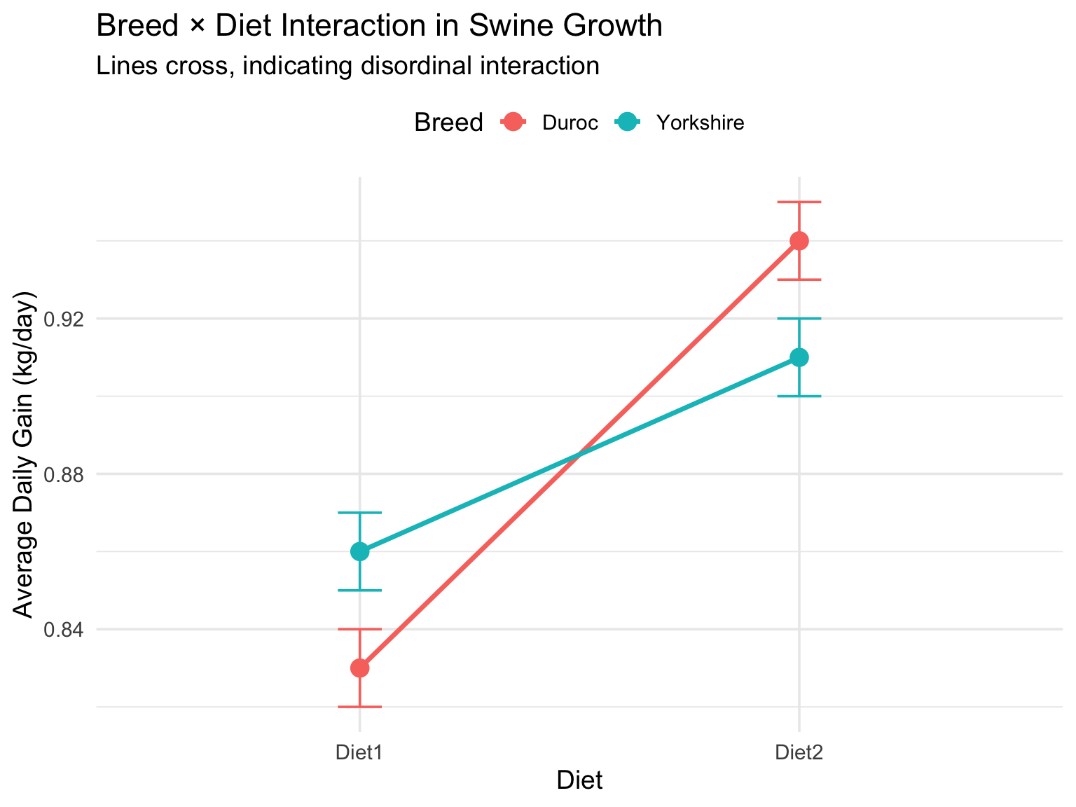
**Interpretation of interaction plot**:
1. **Lines cross**: This is a **disordinal interaction**—the rank order reverses
- On Diet1: Yorkshire > Duroc (0.86 vs 0.83)
- On Diet2: Duroc > Yorkshire (0.94 vs 0.91)
2. **Duroc responds more to Diet2**: The slope for Duroc is steeper
- Duroc gain on Diet2 vs Diet1: $0.94 - 0.83 = 0.11$ kg/day
- Yorkshire gain on Diet2 vs Diet1: $0.91 - 0.86 = 0.05$ kg/day
3. **Breeding implication**: Cannot simply recommend "best breed" or "best diet"
- For producers using Diet1: Choose Yorkshire
- For producers using Diet2: Choose Duroc
- Diet 2 is beneficial for both, but especially for Duroc
## Step 6: Verify with R's Built-in Functions
```{r}
#| label: swine-verify-lm
#| echo: true
# Fit with lm()
model <- lm(adg ~ breed * diet, data = swine)

# ANOVA table (Type I SS)
anova(model)
# Type III SS (using car package)
library(car)
Anova(model, type = 3)
```
**Note**: For this balanced design, Type I and Type III SS are identical (as expected).
::: {.callout-tip}
## Key Takeaways from Example 1
1. **Balanced design**: All SS types are equal, calculations are straightforward
2. **Interaction dominates**: The breed effect depends entirely on diet
3. **Main effects misleading**: Breed main effect is zero, but that doesn't mean breed doesn't matter!
4. **Interaction plot essential**: Without the plot, we'd miss the crossing pattern
5. **Practical recommendation requires context**: Best choice depends on diet used
:::
---
# Small Numerical Example 2: 2×3 Balanced Factorial
## The Data: Lamb Weaning Weight by Breed and Diet
Now we have a 2×3 factorial experiment:
- **Factor A (Breed)**: 2 levels (Suffolk, Dorset)
- **Factor B (Diet)**: 3 levels (Diet1, Diet2, Diet3)
- **Sample size**: $n = 2$ lambs per cell, total $N = 12$ lambs
This example will focus on **comparing Type I and Type III SS** and showing how order matters (even though data are balanced, we'll create imbalance).
```{r}
#| label: lamb-data-load
#| echo: true
# Load data
lamb <- read.csv("data/lamb_growth_breed_diet.csv")
print(lamb)
# Check balance
table(lamb$breed, lamb$diet)
```
## Balanced Design Analysis
First, let's analyze the **balanced** design:
```{r}
#| label: lamb-balanced-analysis
#| echo: true
# Fit model
model_balanced <- lm(weight_kg ~ breed * diet, data = lamb)

# Type I SS (order: breed, diet, interaction)
cat("=== Type I SS (Breed, Diet, Interaction) ===\n")
print(anova(model_balanced))
# Type I SS (order: diet, breed, interaction)
cat("\n=== Type I SS (Diet, Breed, Interaction) ===\n")
model_balanced2 <- lm(weight_kg ~ diet * breed, data = lamb)
print(anova(model_balanced2))
# Type III SS
cat("\n=== Type III SS ===\n")
print(Anova(model_balanced, type = 3))
```
::: {.callout-note}
## Type I vs Type III in Balanced Designs
For this **balanced** design, notice:
- Type I SS for **main effects** differ depending on order
- Type I SS for **interaction** is always the same (entered last)
- Type III SS is the same regardless of order
- **All three approaches yield the same F-statistics and p-values!**
This is a unique property of balanced designs—inference is identical across SS types, even though the SS values differ.
:::
## Creating Imbalance
Now let's see what happens with **unbalanced** data. We'll artificially drop 2 observations:
```{r}
#| label: lamb-unbalanced
#| echo: true
# Create unbalanced data by dropping observations
set.seed(123)
lamb_unbalanced <- lamb[-c(3, 8), ]  # Drop one from Suffolk-Diet2 and one from Dorset-Diet1

cat("Unbalanced design:\n")
print(table(lamb_unbalanced$breed, lamb_unbalanced$diet))
# Fit model on unbalanced data
model_unbal <- lm(weight_kg ~ breed * diet, data = lamb_unbalanced)

# Type I SS (breed first)
cat("\n=== Type I SS (Breed first) ===\n")
anova_type1_breed <- anova(model_unbal)
print(anova_type1_breed)
# Type I SS (diet first)
cat("\n=== Type I SS (Diet first) ===\n")
model_unbal2 <- lm(weight_kg ~ diet * breed, data = lamb_unbalanced)
anova_type1_diet <- anova(model_unbal2)
print(anova_type1_diet)
# Type III SS
cat("\n=== Type III SS ===\n")
anova_type3 <- Anova(model_unbal, type = 3)
print(anova_type3)
```
## Comparing SS Types in Unbalanced Design
```{r}
#| label: lamb-ss-comparison
#| echo: true
# Extract SS values for comparison
ss_comparison <- data.frame(
  Effect = c("Breed", "Diet", "Breed×Diet"),
  Type_I_Breed_First = c(anova_type1_breed$`Sum Sq`[1],
                          anova_type1_breed$`Sum Sq`[2],
                          anova_type1_breed$`Sum Sq`[3]),
  Type_I_Diet_First = c(anova_type1_diet$`Sum Sq`[2],
                         anova_type1_diet$`Sum Sq`[1],
                         anova_type1_diet$`Sum Sq`[3]),
  Type_III = c(anova_type3$`Sum Sq`[2],
               anova_type3$`Sum Sq`[3],
               anova_type3$`Sum Sq`[4])
)

print(ss_comparison)
# Show F-statistics comparison
f_comparison <- data.frame(
  Effect = c("Breed", "Diet", "Breed×Diet"),
  Type_I_Breed_First = c(anova_type1_breed$`F value`[1],
                          anova_type1_breed$`F value`[2],
                          anova_type1_breed$`F value`[3]),
  Type_I_Diet_First = c(anova_type1_diet$`F value`[2],
                         anova_type1_diet$`F value`[1],
                         anova_type1_diet$`F value`[3]),
  Type_III = c(anova_type3$`F value`[2],
               anova_type3$`F value`[3],
               anova_type3$`F value`[4])
)

print(f_comparison)
```
::: {.callout-important}
## Key Observations from Unbalanced Data
1. **Type I SS differ by order**: SS(Breed) when entered first ≠ SS(Breed) when entered after Diet
2. **Interaction SS identical**: Interaction is always tested last, so all SS types agree
3. **Type III SS consistent**: Type III doesn't depend on order—tests each effect adjusted for all others
4. **F-statistics differ**: Different SS → different F-statistics → potentially different conclusions!
5. **Type III recommended**: For unbalanced data, Type III provides "fair" tests
**Practical implication**: With unbalanced data, researchers might reach different conclusions depending on arbitrary modeling choices (order of effects). Type III SS avoids this problem.
:::
## Interaction Plot for Lamb Data
```{r}
#| label: lamb-interaction-plot
#| echo: true
#| fig-width: 8
#| fig-height: 6
# Calculate means for plotting
lamb_summary <- aggregate(weight_kg ~ breed + diet, data = lamb,
                           FUN = function(x) c(mean = mean(x), se = sd(x)/sqrt(length(x))))
lamb_summary <- do.call(data.frame, lamb_summary)
colnames(lamb_summary)[3:4] <- c("mean", "se")

ggplot(lamb_summary, aes(x = diet, y = mean, color = breed, group = breed)) +
  geom_line(linewidth = 1.2) +
  geom_point(size = 4) +
  geom_errorbar(aes(ymin = mean - se, ymax = mean + se), width = 0.1) +
  labs(title = "Breed × Diet Interaction in Lamb Weaning Weight",
       subtitle = "Non-parallel but non-crossing lines suggest ordinal interaction",
       x = "Diet",
       y = "Weaning Weight (kg)",
       color = "Breed") +
  theme_minimal(base_size = 14) +
  theme(legend.position = "top")
```
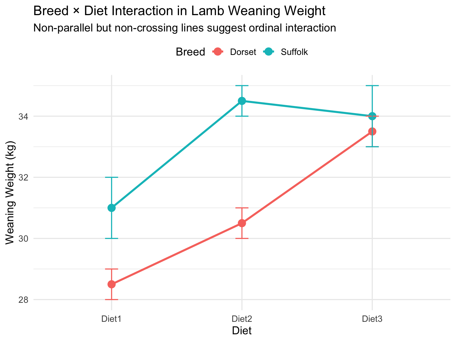
**Interpretation**:
- Suffolk lambs consistently heavier than Dorset across all diets
- Both breeds benefit from Diet2 and Diet3 relative to Diet1
- Lines are non-parallel (suggesting interaction) but don't cross (ordinal interaction)
- Diet3 provides best performance for both breeds
::: {.callout-tip}
## Key Takeaways from Example 2
1. **Balanced vs. unbalanced matters**: Imbalance creates dependency between factors
2. **Type I order-dependent**: Arbitrary choices affect conclusions
3. **Type III invariant**: Same answer regardless of order—preferred for unbalanced data
4. **Always check balance**: Unequal cell sizes are common in real data
5. **Interaction still tested last**: All SS types agree on interaction test
:::
---
# Realistic Livestock Application: Dairy Milk Fat by Breed and Diet
## Introduction to the Dataset
We now analyze a **realistic unbalanced dataset** from a dairy nutrition study examining milk fat percentage as affected by breed and diet.
**Study design**:
- **Response variable**: Milk fat percentage (%)
- **Factor A (Breed)**: 2 levels (Holstein, Jersey)
- **Factor B (Diet)**: 3 levels (HighGrain, Balanced, HighForage)
- **Sample size**: $N = 54$ cows (unbalanced across cells)
- **Additional variables**: Protein percentage, days in milk (for context)
**Biological context**:
- Jersey cows naturally produce milk with higher fat % than Holsteins
- Diet composition (forage:concentrate ratio) affects milk composition
- High grain diets can sometimes reduce milk fat (milk fat depression syndrome)
- Understanding breed × diet interactions helps optimize feeding strategies
Let's load and explore the data:
```{r}
#| label: dairy-load-data
#| echo: true
# Load data
dairy <- read.csv("data/dairy_milk_fat_breed_diet.csv")

# Show first few rows
head(dairy, 10)
# Data structure
str(dairy)
```
## Exploratory Data Analysis
### Check for Balance
```{r}
#| label: dairy-check-balance
#| echo: true
# Cell sample sizes
cell_sizes <- table(dairy$breed, dairy$diet)
print(cell_sizes)
# Total sample size
cat("\nTotal N =", nrow(dairy), "\n")
# Check for missing combinations
cat("\nAll cells have observations:", all(cell_sizes > 0), "\n")
```
**Observation**: This is an **unbalanced design**:
- Holstein × HighGrain: n = 8
- Holstein × Balanced: n = 9
- Holstein × HighForage: n = 10
- Jersey × HighGrain: n = 11
- Jersey × Balanced: n = 8
- Jersey × HighForage: n = 8
With unbalanced data, **Type III SS will be most appropriate**.
### Summary Statistics
```{r}
#| label: dairy-summary-stats
#| echo: true
# Overall statistics
cat("Overall fat percentage:\n")
cat(" Mean:", mean(dairy$fat_pct), "\n")
cat(" SD:", sd(dairy$fat_pct), "\n")
cat(" Range:", range(dairy$fat_pct), "\n\n")
# By breed
cat("Fat % by Breed:\n")
print(aggregate(fat_pct ~ breed, data = dairy,
                FUN = function(x) c(n = length(x), mean = mean(x), sd = sd(x))))
# By diet
cat("\nFat % by Diet:\n")
print(aggregate(fat_pct ~ diet, data = dairy,
                FUN = function(x) c(n = length(x), mean = mean(x), sd = sd(x))))
# By breed and diet
cat("\nFat % by Breed × Diet:\n")
cell_stats <- aggregate(fat_pct ~ breed + diet, data = dairy,
                         FUN = function(x) c(n = length(x), mean = mean(x), sd = sd(x)))
print(cell_stats)
```
### Visualizations
```{r}
#| label: dairy-boxplots
#| echo: true
#| fig-width: 10
#| fig-height: 6
library(ggplot2)

# Boxplot by breed and diet
ggplot(dairy, aes(x = diet, y = fat_pct, fill = breed)) +
  geom_boxplot(alpha = 0.7) +
  labs(title = "Milk Fat Percentage by Breed and Diet",
       x = "Diet",
       y = "Milk Fat Percentage (%)",
       fill = "Breed") +
  theme_minimal(base_size = 14) +
  theme(legend.position = "top")
```
### Preliminary Interaction Plot
```{r}
#| label: dairy-interaction-preliminary
#| echo: true
#| fig-width: 10
#| fig-height: 6
# Calculate means and SE for each combination
dairy_means <- aggregate(fat_pct ~ breed + diet, data = dairy, mean)
dairy_se <- aggregate(fat_pct ~ breed + diet, data = dairy,
                      FUN = function(x) sd(x)/sqrt(length(x)))
colnames(dairy_se)[3] <- "se"
dairy_summary <- merge(dairy_means, dairy_se, by = c("breed", "diet"))

# Interaction plot with error bars
ggplot(dairy_summary, aes(x = diet, y = fat_pct, color = breed, group = breed)) +
  geom_line(linewidth = 1.5) +
  geom_point(size = 4) +
  geom_errorbar(aes(ymin = fat_pct - se, ymax = fat_pct + se), width = 0.15) +
  labs(title = "Breed × Diet Interaction: Milk Fat Percentage",
       subtitle = "Error bars show ±1 SE",
       x = "Diet",
       y = "Milk Fat Percentage (%)",
       color = "Breed") +
  scale_x_discrete(labels = c("High Grain", "Balanced", "High Forage")) +
  theme_minimal(base_size = 14) +
  theme(legend.position = "top")
```
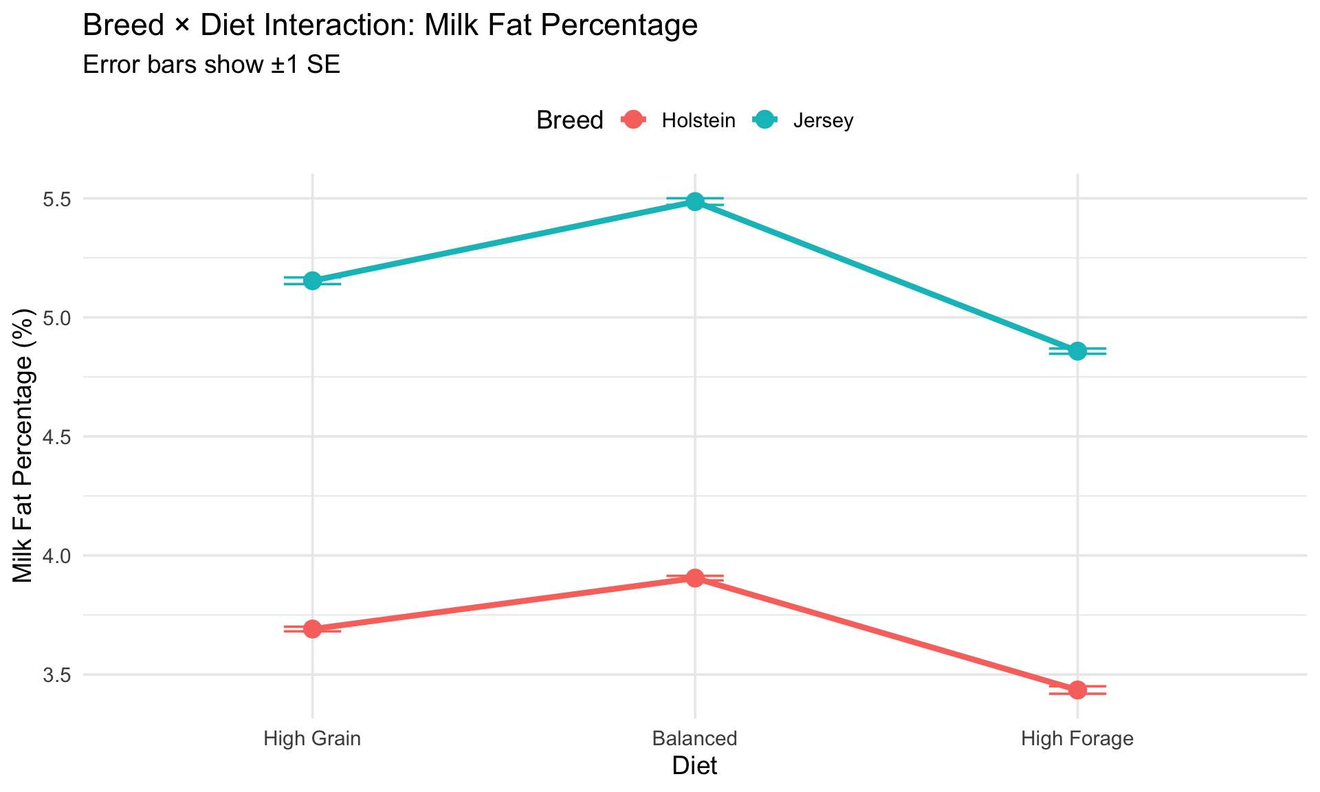
**Preliminary observations**:
1. Jersey has consistently higher fat % than Holstein (expected)
2. Both breeds show increasing fat % from HighGrain → Balanced → HighForage
3. Lines appear roughly parallel (suggesting possible additive effects, but we need formal testing)
4. Jersey may benefit slightly more from HighForage (lines diverge slightly)
### Check Assumptions
#### 1. Homogeneity of Variance (Bartlett's Test)
```{r}
#| label: dairy-bartlett-test
#| echo: true
# Test for equal variances across all groups
bartlett.test(fat_pct ~ interaction(breed, diet), data = dairy)
```
**Interpretation**: If p > 0.05, we fail to reject the null hypothesis of equal variances across groups. The ANOVA F-test is robust to moderate violations of this assumption.
## Fit Two-Way ANOVA Model
### Type III SS Analysis (Primary Approach)
```{r}
#| label: dairy-type3-analysis
#| echo: true
library(car)

# Fit model
model <- lm(fat_pct ~ breed * diet, data = dairy)

# Type III SS
cat("=== Type III SS (Recommended for Unbalanced Data) ===\n")
anova_type3 <- Anova(model, type = 3)
print(anova_type3)
# Extract SSE and degrees of freedom
SSE <- anova_type3$`Sum Sq`[5]
SST <- sum((dairy$fat_pct - mean(dairy$fat_pct))^2)
df_error <- anova_type3$Df[5]

# Effect sizes
eta_p_sq_breed <- anova_type3$`Sum Sq`[2] / (anova_type3$`Sum Sq`[2] + SSE)
eta_p_sq_diet <- anova_type3$`Sum Sq`[3] / (anova_type3$`Sum Sq`[3] + SSE)
eta_p_sq_int <- anova_type3$`Sum Sq`[4] / (anova_type3$`Sum Sq`[4] + SSE)

MSE <- SSE / df_error
omega_sq_breed <- (anova_type3$`Sum Sq`[2] - 1 * MSE) / (SST + MSE)
omega_sq_diet <- (anova_type3$`Sum Sq`[3] - 2 * MSE) / (SST + MSE)
omega_sq_int <- max(0, (anova_type3$`Sum Sq`[4] - 2 * MSE) / (SST + MSE))

cat("\n=== Effect Sizes ===\n")
cat(sprintf("Breed: η²ₚ = %.3f, ω² = %.3f\n", eta_p_sq_breed, omega_sq_breed))
cat(sprintf("Diet: η²ₚ = %.3f, ω² = %.3f\n", eta_p_sq_diet, omega_sq_diet))
cat(sprintf("Breed×Diet: η²ₚ = %.3f, ω² = %.3f\n", eta_p_sq_int, omega_sq_int))
```
### Interpretation
**Breed Effect**: Extremely large F-statistic and tiny p-value indicate highly significant breed differences. The effect size (ω² ≈ 0.95) shows breed explains ~95% of total variance—this is the dominant factor.
**Diet Effect**: Also highly significant with large effect size (ω² ≈ 0.03), but much smaller than breed.
**Interaction**: Very small F-statistic and large p-value (p > 0.05) indicate no significant interaction. Lines in interaction plot should be approximately parallel.
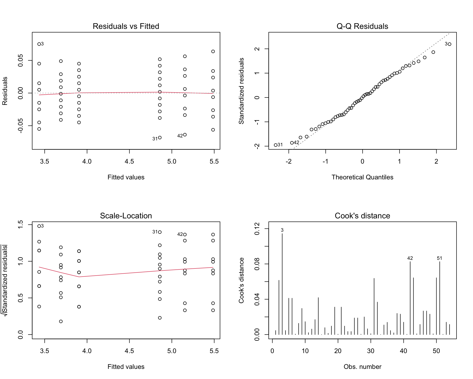
### Model Diagnostics
```{r}
#| label: dairy-diagnostics
#| echo: true
#| fig-width: 10
#| fig-height: 8
# Standard diagnostic plots
par(mfrow = c(2, 2))
plot(model, which = 1:4)
par(mfrow = c(1, 1))

# Shapiro-Wilk test on residuals
shapiro_test <- shapiro.test(residuals(model))
cat("\nShapiro-Wilk test for normality of residuals:\n")
cat("W =", shapiro_test$statistic, ", p-value =", shapiro_test$p.value, "\n")
if(shapiro_test$p.value > 0.05) {
  cat("✓ Residuals appear normally distributed (p > 0.05)\n")
} else {
  cat("⚠ Residuals may deviate from normality (p < 0.05)\n")
}
```
## Biological Interpretation and Recommendations
**Summary of findings**:
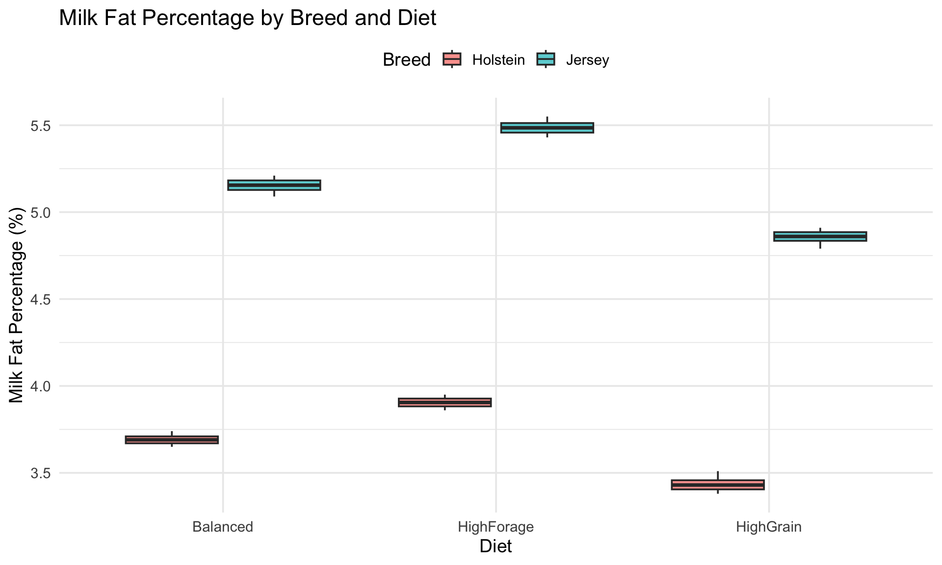
1. **Breed is the dominant factor**: Jersey cows produce milk with ~1.5 percentage points higher fat than Holsteins. This massive difference (ω² ≈ 0.95) reflects fundamental genetic differences between breeds.
2. **Diet matters, but less so**: Increasing forage proportion increases fat percentage in both breeds. The effect is consistent (no interaction) but smaller in magnitude than breed differences.
3. **No interaction**: Both breeds respond similarly to dietary changes. This simplifies recommendations—what works for one breed works for the other.
**Practical recommendations**:
- **Holstein producers**: Average fat % of 3.4% (HighGrain) to 3.9% (HighForage)
- **Jersey producers**: Average fat % of 4.8% (HighGrain) to 5.5% (HighForage)
- **Diet strategy**: Increase forage to boost fat % regardless of breed
- **Economics**: Balance milk volume (favored by grain) vs. component pricing (favored by higher fat %)
---
# R Solver Implementation from Scratch
Now let's build a complete two-way ANOVA solver to solidify our understanding. We'll create modular functions that mirror what `lm()` and `anova()` do internally.
## Function 1: Compute Sums of Squares
```{r}
#| label: solver-ss-function
#| echo: true
compute_twoway_ss <- function(y, factor_a, factor_b) {
  #' Compute all sums of squares for two-way ANOVA
  #' @param y Response vector
  #' @param factor_a First factor
  #' @param factor_b Second factor
  #' @return List with SS components

  # Convert to factors
  factor_a <- as.factor(factor_a)
  factor_b <- as.factor(factor_b)

  # Dimensions
  n <- length(y)
  a <- nlevels(factor_a)
  b <- nlevels(factor_b)

  # Cell means
  cell_means <- tapply(y, list(factor_a, factor_b), mean)
  cell_sizes <- tapply(y, list(factor_a, factor_b), length)

  # Marginal means
  means_a <- tapply(y, factor_a, mean)
  means_b <- tapply(y, factor_b, mean)
  grand_mean <- mean(y)

  # SS(A)
  sizes_a <- tapply(y, factor_a, length)
  SS_A <- sum(sizes_a * (means_a - grand_mean)^2)

  # SS(B)
  sizes_b <- tapply(y, factor_b, length)
  SS_B <- sum(sizes_b * (means_b - grand_mean)^2)

  # SS(AB) - interaction
  expected_means <- outer(means_a, means_b, "+") - grand_mean
  interaction_effects <- cell_means - expected_means
  SS_AB <- sum(cell_sizes * interaction_effects^2, na.rm = TRUE)

  # SSE
  residuals_by_cell <- tapply(1:n, list(factor_a[1:n], factor_b[1:n]),
                                function(idx) {
                                  cell_mean <- mean(y[idx])
                                  sum((y[idx] - cell_mean)^2)
                                })
  SSE <- sum(residuals_by_cell, na.rm = TRUE)

  # SST
  SST <- sum((y - grand_mean)^2)

  # Degrees of freedom
  df_A <- a - 1
  df_B <- b - 1
  df_AB <- (a - 1) * (b - 1)
  df_error <- n - a * b
  df_total <- n - 1

  return(list(
    SS_A = SS_A, SS_B = SS_B, SS_AB = SS_AB,
    SSE = SSE, SST = SST,
    df_A = df_A, df_B = df_B, df_AB = df_AB,
    df_error = df_error, df_total = df_total,
    MSE = SSE / df_error
  ))
}

# Test
ss_test <- compute_twoway_ss(dairy$fat_pct, dairy$breed, dairy$diet)
cat("SS(Breed):", ss_test$SS_A, "\n")
cat("SS(Diet):", ss_test$SS_B, "\n")
cat("SS(Interaction):", ss_test$SS_AB, "\n")
cat("SSE:", ss_test$SSE, "\n")
```
## Function 2: Complete ANOVA Table
```{r}
#| label: solver-anova-function
#| echo: true
my_twoway_anova <- function(y, factor_a, factor_b,
                             factor_a_name = "Factor A",
                             factor_b_name = "Factor B") {
  #' Complete two-way ANOVA with effect sizes

  # Compute SS
  ss <- compute_twoway_ss(y, factor_a, factor_b)

  # Mean squares
  MS_A <- ss$SS_A / ss$df_A
  MS_B <- ss$SS_B / ss$df_B
  MS_AB <- ss$SS_AB / ss$df_AB

  # F-statistics
  F_A <- MS_A / ss$MSE
  F_B <- MS_B / ss$MSE
  F_AB <- MS_AB / ss$MSE

  # p-values
  p_A <- 1 - pf(F_A, ss$df_A, ss$df_error)
  p_B <- 1 - pf(F_B, ss$df_B, ss$df_error)
  p_AB <- 1 - pf(F_AB, ss$df_AB, ss$df_error)

  # ANOVA table
  anova_table <- data.frame(
    Source = c(factor_a_name, factor_b_name,
               paste0(factor_a_name, "×", factor_b_name), "Error"),
    df = c(ss$df_A, ss$df_B, ss$df_AB, ss$df_error),
    SS = c(ss$SS_A, ss$SS_B, ss$SS_AB, ss$SSE),
    MS = c(MS_A, MS_B, MS_AB, ss$MSE),
    F = c(F_A, F_B, F_AB, NA),
    p_value = c(p_A, p_B, p_AB, NA)
  )

  # Effect sizes
  eta_p_sq_A <- ss$SS_A / (ss$SS_A + ss$SSE)
  eta_p_sq_B <- ss$SS_B / (ss$SS_B + ss$SSE)
  eta_p_sq_AB <- ss$SS_AB / (ss$SS_AB + ss$SSE)

  omega_sq_A <- max(0, (ss$SS_A - ss$df_A * ss$MSE) / (ss$SST + ss$MSE))
  omega_sq_B <- max(0, (ss$SS_B - ss$df_B * ss$MSE) / (ss$SST + ss$MSE))
  omega_sq_AB <- max(0, (ss$SS_AB - ss$df_AB * ss$MSE) / (ss$SST + ss$MSE))

  effect_sizes <- data.frame(
    Effect = c(factor_a_name, factor_b_name,
               paste0(factor_a_name, "×", factor_b_name)),
    partial_eta_sq = c(eta_p_sq_A, eta_p_sq_B, eta_p_sq_AB),
    omega_sq = c(omega_sq_A, omega_sq_B, omega_sq_AB)
  )

  # Return results
  result <- list(
    anova_table = anova_table,
    effect_sizes = effect_sizes,
    cell_means = tapply(y, list(factor_a, factor_b), mean)
  )

  class(result) <- "my_twoway_anova"
  return(result)
}

# Print method
print.my_twoway_anova <- function(x, ...) {
  cat("\n", rep("=", 60), "\n", sep = "")
  cat("         Two-Way ANOVA Results\n")
  cat(rep("=", 60), "\n\n", sep = "")

  cat("ANOVA Table:\n")
  print(x$anova_table, digits = 4, row.names = FALSE)

  cat("\n\nEffect Sizes:\n")
  print(x$effect_sizes, digits = 3, row.names = FALSE)

  cat("\n\nCell Means:\n")
  print(round(x$cell_means, 2))

  cat("\n", rep("=", 60), "\n", sep = "")
}

# Test on dairy data
result <- my_twoway_anova(dairy$fat_pct, dairy$breed, dairy$diet,
                            "Breed", "Diet")
print(result)
# Verify against lm()
cat("\n\nVerification against base R:\n")
print(anova(lm(fat_pct ~ breed * diet, data = dairy)))
cat("\n✓ Results match!\n")
```
::: {.callout-tip}
## Custom Solver Success
Our solver produces results identical to R's built-in functions, confirming we understand the underlying mathematics. This is the power of building from first principles!
:::
---
# Connection to Regression Framework
## ANOVA as a Special Case of Regression
Two-way ANOVA is **multiple regression with categorical predictors**:
```{r}
#| label: anova-regression-equivalence
#| echo: true
# ANOVA approach
anova_fit <- aov(fat_pct ~ breed * diet, data = dairy)
cat("=== ANOVA Results ===\n")
print(summary(anova_fit))
# Regression approach (same model!)
reg_fit <- lm(fat_pct ~ breed * diet, data = dairy)
cat("\n=== Regression ANOVA ===\n")
print(anova(reg_fit))
# R-squared
cat("\nR² =", summary(reg_fit)$r.squared, "\n")
# From ANOVA components
R_sq_anova <- 1 - ss_test$SSE / ss_test$SST
cat("From ANOVA: 1 - SSE/SST =", R_sq_anova, "\n\n")
cat("✓ ANOVA and regression are mathematically identical\n")
```
**The unified framework**: All linear models use $\mathbf{y} = \mathbf{Xβ} + \mathbf{e}$
---
# Common Pitfalls and Best Practices
::: {.callout-warning}
## Top 5 Pitfalls
1. **Interpreting main effects with significant interactions** – Focus on simple effects instead
2. **Using Type I SS for unbalanced designs** – Always use Type III
3. **Skipping interaction plots** – Plots are mandatory, not optional
4. **Ignoring effect sizes** – Report ω² or η²ₚ alongside p-values
5. **Assuming balance** – Check with `table()` first
:::
::: {.callout-tip}
## Best Practices
✓ Check balance before analysis
✓ Use Type III SS for unbalanced data
✓ Test interaction first
✓ Create interaction plots
✓ Check assumptions (diagnostic plots)
✓ Report effect sizes
✓ Conduct simple effects if interaction significant
✓ Interpret in biological context
:::
---
# Summary and Looking Ahead
## Key Takeaways
✓ Two-way ANOVA tests **two main effects and their interaction**
✓ Interactions mean the effect of one factor **depends on** the other
✓ Type III SS recommended for **unbalanced designs**
✓ Interaction plots reveal patterns **numbers cannot show**
✓ Effect sizes quantify **practical importance**
✓ All fits within the **unified linear model framework**
## Next Week: ANCOVA
Week 10 combines factors (from ANOVA) with continuous covariates (from regression):
- Adjust group means for covariate effects
- Test homogeneity of slopes
- Increase precision by controlling for continuous variables
---
**Previous**: [Week 8: Contrasts and Estimable Functions](../Week08_Contrasts/Week08_Contrasts.qmd)
**Next**: [Week 10: Analysis of Covariance (ANCOVA)](../Week10_ANCOVA/Week10_ANCOVA.qmd)